Showing posts with label new homework problem. Show all posts

Friday, December 27, 2024

The Cyclotron Resonance Hypothesis

Intermediate Physics for Medicine and Biology
Want a sneak peek at one of the new homework problems tentatively included in the 6th edition of Intermediate Physics for Medicine and Biology? Today I present a problem related to the flawed “cyclotron resonance hypothesis.” A lot of nonsense has been written about the idea of extremely low frequency electromagnetic fields influencing biology and medicine, and one of the proposed mechanisms for such effects is cyclotron resonance. 

In Section 8.1 of the 5th edition of IPMB, Russ Hobbie and I discuss the cyclotron.

One important application of magnetic forces in medicine is the cyclotron. Many hospitals have a cyclotron for the production of radiopharmaceuticals, especially for generating positron-emitting nuclei for use in Positron EmissionTomography (PET) imaging (see Chap. 17).

Consider a particle of charge q and mass m, moving with speed v in a direction perpendicular to a magnetic field B. The magnetic force will bend the path of the particle into a circle. Newton’s second law states that the mass times the centripetal acceleration, v2/r, is equal to the magnetic force

      mv2/r = qvB.      (8.5)

The speed is equal to [the] circumference of the circle, 2πr, divided by the period of the orbit, T. Substituting this expression for v into Eq. (8.5) and simplifying, we find

       T = 2π m/(qB).   (8.6)

In a cyclotron particles orbit at the cyclotron frequency, f = 1/T. Because the magnetic force is perpendicular to the motion, it does not increase the particles’ speed or energy. To do that, the particles are subjected periodically to an electric field that changes direction with the cyclotron frequency so that it is always accelerating, not decelerating, the particles. This would be difficult if not for the fortuitous disappearance of both v and r from Eq. (8.6), so that the cyclotron frequency only depends on the charge-to-mass ratio of the particles and the magnetic field, but not on their energy.

This analysis of cyclotron motion works great in a vacuum. The trouble begins when you apply the cyclotron concept to ions in the conducting fluids of the body. The proposed hypothesis says that when an ion is moving about in the presence of the earth’s magnetic field, the resulting magnetic force causes it to orbit about the magnetic field lines, with an orbital period equal to the reciprocal of the cyclotron frequency. If any electric field is present at that same frequency, it could interact with the ion, increasing its energy or causing it to cross the cell membrane.

Below is a draft of the new homework problem, which I hope debunks this erroneous hypothesis.

Section 9.1

Problem 7. One mechanism for how organisms are influenced by extremely low frequency electric fields is the cyclotron resonance hypothesis. 

(a) The strength of the earth's magnetic field is about 5 × 10⁻⁵ T. A calcium ion has a mass of 6.7 × 10⁻²⁶ kg and a charge of 3.2 × 10⁻¹⁹ C. Calculate the cyclotron frequency of the calcium ion. If an electric field exists in the tissue at that frequency, the calcium ion will be in resonance with the cyclotron frequency, which could magnify any biological effect. 

(b) This mechanism seems to provide a way for an extremely low frequency electric field to interact with calcium ions, and calcium influences many cellular processes. But consider this hypothesis in more detail. Use Eq. 4.12 to calculate the root-mean-square speed of a calcium ion at body temperature. Use this speed in Eq. 8.5 to calculate the radius of the orbit. Compare this to the size of a typical cell. 

(c) Now make a similar analysis, but assume the radius of the calcium ion orbit is about the size of a cell (since it would have difficulty crossing the cell membrane). Then use this radius in Eq. 8.5 to determine the speed of the calcium ion. If this is the root-mean-square speed, what is the body temperature? 

(d) Finally, compare the period of the orbit to the time between collisions of the calcium ion with a water molecule. What does this imply for the orbit?

This analysis should convince you that the cyclotron resonance hypothesis is unlikely to be correct. Although the frequency is reasonable, the orbital radius will be huge unless the ions are traveling extraordinarily slowly. Collisions with water molecules will completely disrupt the orbit.

For those who don't have the 5th edition of IPMB handy, Eq. 4.12 says the root-mean-square speed is equal to the square root of 3 times Boltzmann's constant times the absolute temperature divided by the mass of the particle. 

I won’t give away the solution to this problem (once the 6th edition of IPMB is out, instructors can get the solution manual for free by emailing me at roth@oakland.edu). But here are some order-of-magnitude results. The cyclotron frequency is tens of hertz. The root-mean-square (thermal) speed of calcium at body temperature is hundreds of meters per second. The resulting orbital radius is about a meter. That is bigger than the body, and vastly bigger than a cell. To fit the orbit inside a cell, the speed would have to be much slower, on the order of a thousandth of a meter per second, which corresponds to a temperature of about a few nanokelvins. The orbital period is a couple hundredths of a second, but the time between collisions of the ion with a water molecule is one the order of 10–13 seconds, so there are many billions of collisions per orbit. Any circular motion will be destroyed by collisions long before anything like an orbit is established. I’m sorry, but the hypothesis is rubbish.

Are Electromagnetic Fields Making Me Ill? superimposed on Intermediate Physics for Medicine and Biology
Are Electromagnetic Fields
Making Me Ill?

If you want to learn more about how extremely low frequency electric fields interact with tissue, see my book Are Electromagnetic Fields Making Me Ill?

Finally, for you folks who are really on the ball, you may be wondering why this homework problem is listed as being in Chapter 9 when the discussion of the cyclotron is in Chapter 8 of the 5th edition of IPMB. (In this post I changed the equation numbers in the homework problem to match the 5th edition, so you would have them.) Hmm.. is there a new chapter in the 6th edition? More on that later…

 To be fair, I should let my late friend Abraham Liboff tell you his side of the story. In this video, Abe explains how he proposed the cyclotron resonance hypothesis. I liked Abe, but I didn’t like his hypothesis.

https://www.youtube.com/watch?v=YL-wqJ-PMAQ&list=PLCO-VktC6wofkMeEeZknT9Y4WhMnP76Ee&index=6

Friday, August 23, 2024

The Song of the Dodo

The Song of the Dodo,
by David Quammem.
One of my favorite science writers is David Quammen. I’ve discussed several of his books in this blog before, such as Breathless, Spillover, and The Tangled Tree. A copy of one of his earlier books—The Song of the Dodo: Island Biogeography in an Age of Extinctions—has sat on my bookshelf for a while, but only recently have I had a chance to read it. I shouldn’t have waited so long. It’s my favorite.

Quammen is not surprised that the central idea of biology, natural selection, was proposed by two scientists who studied islands: Charles Darwin and the Galapagos, and Alfred Russell Wallace and the Malay Archipelago. The book begins by telling Wallace’s story. Quammen calls him “the man who knew islands.” Wallace was the founder of the science of biogeography: the study of how species are distributed throughout the world. For example, Wallace’s line lies between two islands in Indonesia that are only 20 miles apart: Bali (with plants and animals similar to those native to Asia) and Lombok (with flora and fauna more like that found in Australia). Because islands are so isolated, they are excellent laboratories for studying speciation (the creation of new species through evolution) and extinction (the disappearance of existing species).

Quammen is the best writer about evolution since Stephen Jay Gould. I would say that Gould was better at penning essays and Quammen is better at authoring books. Much of The Song of the Dodo deals with the history of science. I would rank it up there with my favorite history of science books: The Making of the Atomic Bomb by Richard Rhodes, The Eighth Day of Creation by Horace Freeland Judson, and The Maxwellians by Bruce Hunt.

Yet, The Song of the Dodo is more than just a history. It’s also an amazing travelogue. Quammen doesn’t merely write about islands. He visits them, crawling through rugged jungles to see firsthand animals such as the Komodo Dragon (a giant man-eating lizard), the Madagascan Indri (a type of lemur), and the Thylacine (a marsupial also known as the Tasmanian tiger). A few parts of The Song of the Dodo are one comic sidekick away from sounding like a travel book Tony Horwitz might have written. Quammen talks with renowned scientists and takes part in their research. He reminds me of George Plimpton, sampling different fields of science instead of trying out various sports.

Although I consider myself a big Quammen fan, he does have one habit that bugs me. He hates math and assumes his readers hate it too. In fact, if Quammen’s wife Betsy wanted to get rid of her husband, she would only need to open Intermediate Physics for Medicine and Biology to a random page and flash its many mathematical equations in front of his face. It would put him into shock, and he probably wouldn’t last the hour. In his book, Quammen only presents one equation and apologizes profusely for it. It’s a power law relationship

S = c An .

This is the same equation that Russ Hobbie and I analyze in Chapter 2 of IPMB, when discussing log-log plots and scaling. How do you determine the dimensionless exponent n for a particular case? As is my wont, I’ll show you in a new homework problem.
Section 2.11

Problem 40½. In island biogeography, the number of species on an island, S, is related to the area of the island, A, by the species-area relationship: S = c An, where c and n are constants. Philip Darlington counted the number of reptile and amphibian species from several islands in the Antilles. He found that when the island area increased by a factor of ten, the number of species doubled. Determine the value of n.
Let me explain to mathaphobes like Quammen how to solve the problem. Assume that on one island there are S0 species and the area is A0. On another island, there are 2S0 species and an area of 10A0. Put these values into the power law to find S0 = cA0n and 2S0 = c(10A0)n. Now divide the second equation by the first (c, S0, and A0 all cancel) to find 2 = 10n. Take the logarithm of both sides, so log(2) = log(10n), or using a property of logarithms log(2) = n log(10). So n = log(2)/log(10) = 0.3. Note that n is positive, as it should be since increasing the area increases the number of species.

When I finished the main text of The Song of the Dodo, I thumbed through the glossary and found an entry for logarithm. “Aww,” I thought, “Quammen was only joking; he likes math after all.” Then I read his definition: “logarithm. A mathematical thing. Never mind.”

About halfway through, the book makes a remarkable leap from island biogeography—interesting for its history and relevance to exotic tropical isles—to mainland ecology, relevant to critical conservation efforts. Natural habitats on the continents are being broken up into patches, a process called fragmentation. The expansion of towns and farms creates small natural reserves surrounded by inhospitable homes and fields. The few remaining native regions tend to be small and isolated, making them similar to islands. A small natural reserve cannot support the species diversity that a large continent can (S = c An). Extinctions inevitably follow.

The Song of the Dodo also provides insight into how science is done. For instance, the species-area relationship was derived by Robert MacArthur and Edward Wilson. While it’s a valuable contribution to island biogeography, scientists disagree on its applicability to fragmented continents, and in particular they argue about its relevance to applied conservation. Is a single large reserve better than several small ones? In the 1970s a scientific battle raged, with Jared Diamond supporting a narrow interpretation of the species-area relationship and Dan Simberloff advocating for a more nuanced and less dogmatic view. As in any science, the key is to get data to test your hypothesis. Thomas Lovejoy performed an experiment in the Amazon to test the species-area relationship. Parts of the rainforest were being cleared for agriculture or other uses, but the Brazilian government insisted on preserving some of the native habitat. Lovejoy obtained permission to create many different protected rainforest reserves, each a different size. His team monitored the reserves before and after they became isolated from adjacent lands, and tracked the number of species supported in each of these “islands” over time. While the results are complicated, there is a correlation between species diversity and reserve size. Area matters.

One theme that runs through the story is extinction. If you read the book, you better have your hanky ready when you reach the part where Quammen imagines the death of the last Dodo bird. Conservation efforts are featured throughout the text, such as the quest to save the Mauritius kestrel.  
 
The Song of the Dodo concludes with a mix of optimism and pessimism. Near the end of the book, when writing about his trip to Aru (an island in eastern Indonesia) to observe a rare Bird of Paradise, Quammen writes
The sad, dire things that have happened elsewhere, in so many parts of the world—biological imperialism, massive habitat destruction, fragmentation, inbreeding depression, loss of adaptability, decline of wild populations to unviable population levels, ecosystem decay, trophic cascades, extinction, extinction, extinction—haven’t yet happened here. Probably they soon will. Meanwhile, though, there’s still time. If time is hope, there’s still hope.

An interview with David Quammen, by www.authorsroad.com

https://www.youtube.com/watch?v=Quq7PNH1zWM

Friday, May 31, 2024

Can the Microwave Auditory Effect Be ‘Weaponized’

Can the Microwave Auditory
Effect be Weaponized?”
I was recently reading Ken Foster, David Garrett, and Marvin Ziskin’s paper “Can the Microwave Auditory Effect Be Weaponized?” (Frontiers in Public Health, Volume 9, 2021). It analyzed if microwave weapons could be used to “attack” diplomats and thereby cause the Havana syndrome. While I am interested in the Havana syndrome (I discussed it in my book Are Electromagnetic Fields Making Me Ill?), today I merely want to better understand Foster et al.’s proposed mechanism by which an electromagnetic wave can induce an acoustic wave in tissue.

As is my wont, I will present this mechanism as a homework problem at a level you might find in Intermediate Physics for Medicine and Biology. I’ll assign the problem to Chapter 13 about Sound and Ultrasound, although it draws from several chapters.

Forster et al. represent the wave as decaying exponentially as it enters the tissue, with a skin depth λ. To keep things simple and to focus of the mechanism rather than the details, I’ll assume the energy in the electromagnetic wave is absorbed uniformly in a thin layer of thickness λ, ignoring the exponential behavior.

Section 13.4
Problem 17 ½. Assume an electromagnetic wave of intensity I0 (W/m2) with area A (m2) and duration τ (s) is incident on tissue. Furthermore, assume all its energy is absorbed in a depth λ (m).

(a) Derive an expression for the energy E (J) dissipated in the tissue.

(b) Derive an expression for the tissue’s increase in temperature ΔT (°C), E = C ΔT, where C (J/°C) is the heat capacity. Then express C in terms of the specific heat capacity c (J/°C kg), the density ρ (kg/m3), and the volume where the energy was deposited V (m3). (For a discussion of the heat capacity, see Sec. 3.11).

(c) Derive an expression for the fractional increase in volume, ΔV/V, caused by the increase in temperature, ΔV/V = αΔT, where α (1/°C) is the tissue’s coefficient of thermal expansion.

(d) Derive an expression for the change in pressure, ΔP (Pa), caused by this fractional change in volume, ΔP = B ΔV/V, where B (Pa) is the tissue’s bulk modulus. (For a discussion of the bulk modulus, see Sec. 1.14).

(e) You expression in part d should contain a factor Bα/. Show that this factor is dimensionless. It is called the Grüneisen parameter.

(f) Assume α = 0.0003 1/°C, B = 2 × 10⁹ Pa, c = 4200 J/kg °C, and ρ = 1000 kg/m3. Evaluate the Grüneisen parameter. Calculate the change in pressure ΔP if the intensity is 10 W/m2, the skin depth is 1 mm, and the duration is 1 μs.

I won’t solve the entire problem for you, but the answer for part d is

                            ΔPI0 (τ/λ) [/] .

I should stress that this calculation is approximate. I ignored the exponential falloff. Some of the incident energy could be reflected rather than absorbed. It is unclear if I should use the linear coefficient of thermal expansion or the volume coefficient. The tissue may be heterogeneous. You can probably identify other approximations I’ve made. 

Interestingly, the pressure induced in the tissue varies inversely with the skin depth, which is not what I intuitively expected. As the skin depth gets smaller, the energy is dumped into a smaller volume, which means the temperature increase within this smaller volume is larger. The pressure increase is proportional to the temperature increase, so a thinner skin depth means a larger pressure.

You might be thinking: wait a minute. Heat diffuses. Do we know if the heat would diffuse away before it could change the pressure? The diffusion constant of heat (the thermal diffusivity) D for tissue is about 10-7 m2/s. From Chapter 4 in IPMB, the time to diffuse a distance λ is λ2/D. For λ = 1 mm, this diffusion time is 10 s. For pulses much shorter than this, we can ignore thermal diffusion. 

Perhaps you’re wondering how big the temperature rise is? For the parameters given, it’s really small: ΔT  = 2 × 10–9 °C. This means the fractional change in volume is around 10–12. It’s not a big effect.

The Grüneisen parameter is a dimensionless number. I’m used to thinking of such numbers as being the ratio of two quantities with the same units. For instance, the Reynolds number is the ratio of an inertial force to a viscous force, and the Péclet number is the ratio of transport by drift to transport by diffusion. I’m having trouble interpreting the Grüneisen parameter in this way. Perhaps it has something to do with the ratio of thermal energy to elastic energy, but the details are not obvious, at least not to me.

What does this all have to do with the Havana syndrome? Not much, I suspect. First, we don’t know if the Havana syndrome is caused by microwaves. As far as I know, no one has ever observed microwaves associated with one of these “attacks” (perhaps the government has but they keep the information classified). This means we don’t know what intensity, frequency (and thus, skin depth), and pulse duration to assume. We also don’t know what pressure would be required to explain the “victim’s” symptoms. 

In part f of the problem, I used for the intensity the upper limit allowed for a cell phone, the skin depth corresponding approximately to a microwave frequency of about ten gigahertz, and a pulse duration of one microsecond. The resulting pressure of 0.0014 Pa is much weaker than is used during medical ultrasound imaging, which is known to be safe. The acoustic pressure would have to increase dramatically to pose a hazard, which implies very large microwave intensities.

Are Electromagnetic Fields Making Me Ill? superimposed on the cover of Intermediate Physics for Medicine and Biology.
Are Electromagnetic Fields
Making Me Ill?

That such a large intensity electromagnetic wave could be present without being noticeable seems farfetched to me. Perhaps very low pressures could have harmful effects, but I doubt it. I think I’ll stick with my conclusion from Are Electromagnetic Fields Making Me Ill?

Microwave weapons and the Havana Syndrome: I am skeptical about microwave weapons, but so little evidence exists that I want to throw up my hands in despair. My guess: the cause is psychogenic. But if anyone detects microwaves during an attack, I will reconsider.

Friday, December 29, 2023

Special Relativity in IPMB

Electricity and Magnetism, by Edward Purcell, superimposed on Intermediate Physics for Medicine and Biology.
Electricity and Magnetism,
by Edward Purcell.
In Intermediate Physics for Medicine and Biology, Russ Hobbie and I rarely discuss special relativity. We briefly mention that magnetism is a consequence of relativity in Chapter 8 (Biomagnetism) but we don’t develop our study of magnetic fields from this point of view. (If you want to see magnetism analyzed in this way, I suggest looking at the textbook Electricity and Magnetism, by Edward Purcell, which is Volume 2 of the Berkeley Physics Course). We use the relationship between the energy and momentum of a photon, E = pc, in Chapter 15 (Interaction of Photons and Charged Particles with Matter) when analyzing Compton scattering and pair production. And we use Einstein’s famous equation E = mc2, relating a particles energy to its rest mass, when calculating the binding energy of nuclei in Chapter 17 (Nuclear Physics and Nuclear Medicine).

The most relativisticish equation we present is in Chapter 15 when analyzing how charged particles (such as protons, electrons, or alpha particles) lose energy when passing through tissue at relativistic speeds. We write

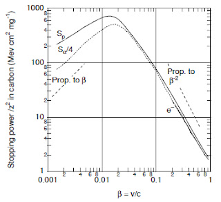
The stopping powers are plotted vs particle speed in the form β = v/c. At low energies (β ≪ 1) β is related to kinetic energy by 


For larger values of β, the relativistically correct expression

was used to convert Fig. 15.17 to 15.18. 

Fig. 15.17


Fig. 15.18

Here’s a new homework problem examining the relationship between a particle’s speed and kinetic energy when its speed is near the speed of light.

Section 15.11

Problem 41 ½. A charged particle’s kinetic energy, T, is related to its mass M and its speed, v. We often express speed in terms of the parameter β = v/c, where c is the speed of light.

(a) At low energies (TMc2, or equivalently β ≪ 1), show that Eq. 15.47 is consistent with the familiar expression from classical mechanics, T = ½ mv2.

(b) Show that Equation 15.48 (the relativistically correct relationship between β and T) reduces to Eq. 15.47 when TMc2.

(c) Plot β versus T/Mc2, both in a linear plot (0 < T/Mc2 < 3) and in a log-log plot (0.0001 < T/Mc2 < 100).

(d) Take a few data points from Fig. 15.17 for a proton, replot them in Fig. 15.18, where the dependent variable is β, not T. See how well they match. Be sure to adjust for the different units for Stopping Power in the two plots.

Friday, May 26, 2023

Terminal Speed of Microorganisms

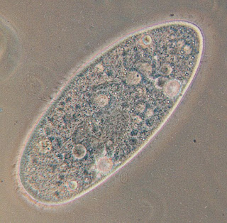
A Paramecium aurelia seen through an optical microscope
A Paramecium aurelia seen through an optical microscope.
Source: Wikipedia (http://en.wikipedia.org/wiki/Image:Paramecium.jpg)

Homework Problem 28 at the end of Chapter 2 in Intermediate Physics for Medicine and Biology asks the reader to calculate the terminal speed of an animal falling in air. Although this problem provides insight, it includes a questionable assumption. Russ and I tell the student to “assume that the frictional force is proportional to the surface area of the animal.” If, however, the animal falls at low Reynolds number, this assumption is not valid. Instead, the drag force is given by Stokes’ law, which is proportional to the radius, not the surface area (radius squared). The new homework problem given below asks the reader to calculate the terminal speed for a microorganism falling through water at low Reynolds number.

Section 2.8

Problem 28 ½. Calculate the terminal speed, V, of a paramecium sinking in water. Assume that the organism is spherical with radius R, and that the Reynolds number is small so that the drag force is given by Stokes’ law. Include the effect of buoyancy. Let the paramecium’s radius be 100 microns and its specific gravity be 1.05. Verify that its Reynolds number is small.
The reader will first need to get the density ρ and viscosity η of water, which are ρ = 1000 kg/m3 and η = 0.001 kg/(m s). The specific gravity is not defined in IPMB, but it’s the density divided by the density of water, implying that the density of the paramecium is 1050 kg/m3. Finally, Stokes’ law is given in IPMB as Eq. 4.17, Fdrag = –6πRηV.

I’ll let you do your own calculation. I calculate the terminal speed to be about 1 mm/s, so it takes about a fifth of a second to sink one body diameter. The Reynolds number is 0.1, which is small, but not exceptionally small.

You should find that the terminal speed increases as the radius squared, in contrast to a drag force proportional to the surface area for which the terminal speed increases in proportion to the radius. Bigger organisms sink faster. The dependence of terminal speed on size is even more dramatic for aquatic microorganisms than for mammals falling in air. To paraphrase Haldane’s quip, “a bacterium is killed, a diatom is broken, a paramecium splashes,” except the speeds are small enough that none of the “wee little beasties” are really killed (the terminal speed is not terminal...get it?) and splashing is a high Reynolds number phenomenon.

Buoyancy is not negligible for aquatic animals. The effective density of a paramecium in air would be about 1000 kg/m3, but in water its effective density drops to a mere 50 kg/m3. Microorganisms are made mostly of water, so they are almost neutrally buoyant. In this homework problem, the effect of gravity is reduced to only five percent of what it would be if buoyancy were ignored.

A paramecium is a good enough swimmer that it can swim upward against gravity if it wants to. Its surface is covered with cilia that beat together like a Roman galley to produce the swimming motion (ramming speed!).

Whenever discussing terminal speed, one should remember that we assume the fluid is initially at rest. In fact, almost any volume of water will have currents moving at speeds greater than 1 mm/s, caused by tides, gravity, thermal convection, wind driven waves, or the wake of a fish swimming by. A paramecium would drift along with these currents. To observe the motion described in this new homework problem, one must be careful to avoid any bulk movement of water.

If you watched a paramecium sink in still water, would you notice any Brownian motion? You can calculate the root-mean-squared thermal speed with Eq. 4.12 in IPMB, using the mass of the paramecium as four micrograms and a temperature of 20° C. You get approximately 0.002 mm/s. That is less than 1% of the terminal speed, so you wouldn’t notice any random Brownian motion unless you measured extraordinarily carefully.

Friday, February 24, 2023

A Simple Mathematical Function Representing the Intracellular Action Potential

In Problem 14 of Chapter 7 in Intermediate Physics for Medicine and Biology, Russ Hobbie and I chose a strange-looking function to represent the intracellular potential along a nerve axon, vi(x). It’s zero everywhere except in the range −a < x < a, where it’s


Why this function? Well, it has several nice properties, which I’ll leave for you to explore in this new homework problem.
Section 7.4

Problem 14 ¼. For the intracellular potential, vi(x), given in Problem 14
(a) show that vi(x) is an even function,
(b) evaluate vi(x) at x = 0,
(c) show that vi(x) and dvi(x)/dx are continuous at x = 0, a/2 and a, and
(d) plot vi(x), dvi(x)/dx, and d2vi(x)/dx2 as functions of x, over the range −2a < x < 2a.
This representation of vi(x) has a shape like that of an action potential. Other functions also have a similar shape, such as a Gaussian. But our function is nice because it’s non-zero over only a finite region (−a < x < a) and it’s represented by a simple, low-order polynomial rather than a special function. An even simpler function for vi(x) would be triangular waveform, like that shown in Figure 7.4 of IPMB. However, that function has a discontinuous derivative and therefore its second derivative is infinite at discrete points (delta functions), making it tricky (but not too tricky) to deal with when calculating the extracellular potential (Eq. 7.21). Our function in Problem 14 ¼ has a discontinuous but finite second derivative.

The main disadvantage of the function in Problem 14 ¼ is that the depolarization phase of the “action potential” has the same shape as the repolarization phase. In a real nerve, the upstroke is usually briefer than the downstroke. The next new homework problem asks you to design a new function vi(x) that does not suffer from this limitation.
Section 7.4

Problem 14 ½. Design a piecewise continuous mathematical function for the intracellular potential along a nerve axon, vi(x), having the following properties. 
(a) vi(x) is zero outside the region −a < x < 2a
(b) vi(x) and its derivative dvi(x)/dx are continuous. 
(c) vi(x) is maximum and equal to one at x = 0. 
(d) vi(x) can be represented by a polynomial bi + ci x + di x2, where i refers to four regions: 
        i = 1,    −a < x < −a/2 
        i = 2, −a/2 < x < 0 
        i = 3,      0 < x < a
        i = 4,      a < x < 2a.
Finally, here’s another function that I’m particularly fond of.
Section 7.4

Problem 14 ¾. Consider a function that is zero everywhere except in the region −a < x < 2a, where it is

(a) Plot vi(x) versus x over the region −a < x < 2a,
(b) Show that vi(x) and its derivative are each continuous. 
(c) Calculate the maximum value of vi(x).
Simple functions like those described in this post rarely capture the full behavior of biological phenomena. Instead, they are “toy models” that build insight. They are valuable tools when describing biological phenomena mathematically.

Friday, December 23, 2022

Think Before You Calculate!

I encourage students to build their qualitative problem solving skills by recasting equations in dimensionless variables, analyzing the limiting behavior of mathematical expressions, and sketching plots showing how functions behave. “Think Before You Calculate!” is my mantra. But how, specifically, do you do this? Let me show you an example.

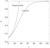
A plot of the solution to the logistic equation.
Fig. 2.16 from IPMB. A plot of the solution
of the logistic equation when y0 = 0.1,
y = 1.0, b0 = 0.0667. Exponential
growth with the same values of
y0 and b0 is also shown.
In Section 2.10 of Intermediate Physics for Medicine and Biology, Russ Hobbie and I discuss the logistic model.
Sometimes a growing population will level off at some constant value. Other times the population will grow and then crash. One model that exhibits leveling off is the logistic model, described by the differential equation

dy/dt = b0 y (1 – y/y) ,                           (2.28)

where b0 and y are constants….

If the initial value of y is y0, the solution of Eq. 2.28 is

y(t) = 1 / [1/y + (1/y0 – 1/y) eb0t] .    (2.29)
Below is a new homework problem, analyzing the logistic equation in a way to build insight. Consider it an early Christmas present. Santa won’t give you the answer, so you need to solve the problem yourself to gain anything from this post.
Section 2.10

Problem 36 ½. Consider the logistic model.

(a) Write Eq. 2.28 in terms of dimensionless variables Y and T, where Y = y/y and T = b0t.

(b) Express the solution Eq. 2.29 in terms of Y, T, and Y0 = y0/y.

(c) Verify that your solution in part (b) obeys the differential equation you derive in part (a).

(d) Verify that your solution in part (b) is equal to Y0 at T = 0.

(e) In a plot of Y(T) versus T, which of the three constants (y, y0, and b0) affect the qualitative shape of the solution, and which just scale the Y and T axes? 

(f) Verify that your solution in part (b) approaches 1 as T goes to infinity.

(g) Find an expression for the slope of the curve Y = Y(T). What is the slope at time T = 0? For what value of Y0 is the initial slope largest? For what values of Y0 is the slope small?

(h) The plot in Fig. 2.16 compares the solution of logistic equation with the exponential Y = Y0 eT. The figure gives the impression that the exponential is a good approximation to the logistic curve at small times. Do the two curves have the same value at T = 0? Do the two curves have the same slope at T = 0?

(i) Sketch plots of Y versus T for Y0 = 0.0001, 0.001, 0.01, and 0.1.

(j) Rewrite the solution from part (b), Y = Y(T), using the constant T0, where T0 = ln[(1−Y0)/Y0]. Show that varying Y0 is equivalent to shifting the solution along the T axis. What value of Y0 corresponds to T0 = 0?

(k) How does the logistic curve behave if Y0 > 1? Sketch a plot of Y versus T for Y0 =1.5.

(l) How does the logistic curve behave if Y0 < 0? Sketch a plot of Y versus T for Y0 = –0.5.

(m) Plot Y versus T for Y0 = 0.1 on semilog graph paper.

If you solve this new homework problem and want to compare you solution to mine, email me at roth@oakland.edu and I’ll send you my solution. 

The Logistic Equation, MIT OpenCourseWare

https://www.youtube.com/watch?v=TCkLSYxx21c&t=69s

Friday, August 19, 2022

The Loudest Sound

In Table 13.1 of Intermediate Physics for Medicine and Biology, Russ Hobbie and I list the approximate intensity levels of various sounds, in decibels. The minimum perceptible sound is 0 dB, a typical office has a sound level of 50 dB, a jack hammer is 100 dB, and the loudest sound listed is a rocket launch pad at 170 dB.

Can there be even louder sounds? Yes, there can! This new homework problem lets you calculate the loudest possible sound.
Section 13.4

Problem 17 ½. Let us calculate the loudest possible sound in air. 
(a) Use Eq. 13.29 to calculate the intensity of a sound in W m−2, using 428 Pa s m−1 for the acoustic impedance of air and one atmosphere (1.01 × 10⁵ Pa) for the pressure. This pressure is the largest that can exist for a sinusoidally varying sound wave, as an even louder sound would create a minimum pressure below zero (less than a vacuum). 
(b) Use the result from part (a) to calculate the intensity in decibels using Eq. 13.34.
For those of you who don’t have a copy of IPMB at your side, here are the two equations you need

                I = ½ p2/Z                                         (13.29)

                Intensity level = 10 log10(I/I0)         (13.34)

where I is the intensity, Z is the acoustic impedance, p is the pressure, I0 is the minimum perceptible intensity (10−12 W m−2), and log10 is the common logarithm.

I’ll let you do the calculation, but you should find that the loudest sound is about 191 dB. Is this really an upper limit? No, you could have a peak pressure larger than one atmosphere, but in that case you wouldn’t be dealing with a traditional sound wave (with pressure ranging symmetrically above and below the ambient pressure) but more of a nonlinear acoustic shock wave.

Krakatoa, by Simon Winchester, superimposed on Intermediate Physics for Medicine and Biology.
Krakatoa,
by Simon Winchester.
Has there ever been a sound that loud? Or, more interestingly, what is the loudest sound ever heard on earth? That’s hard to say for sure, but one possibility is the 1883 eruption of the Krakatoa volcano. We know this sound was loud, because people heard it so far from where the eruption occurred.

Simon Winchester tells this story in his fascinating book Krakatoa: The Day the World Exploded, August 27. 1883. Krakatoa is an island that is now part of Indonesia. When it erupted, people on the island of Rodriguez in the western Indian Ocean, nearly 3000 miles from Krakatoa, could hear it. Winchester writes
In August 1883 the chief of police on Rodriguez was a man named James Wallis, and in his official report… for the month he noted:
On Sunday the 26th the weather was stormy, with heavy rain and squalls; the wind was from SE, blowing with a force of 7 to 10, Beaufort scale. Several times during the night (26th–27th) reports were heard coming from the eastward, like the distant roar of heavy guns. These reports continued at intervals of between three and four hours, until 3 pm on the 27th, and the last two were heard in the directions of Oyster Bay and Port Mathurie [sic].
This was not the roar of heavy guns, however. It was the sound of Krakatoa—busily destroying itself fully 2,968 miles away to the east. By hearing it that night and day, and by noting it down as any good public servant should, Chief Wallis was unknowingly making for himself two quite separate entries in the record books of the future. For Rodriguez Island was the place furthest from Krakatoa where its eruptions could be clearly heard. And the 2,968-mile span that separates Krakatoa and Rodriguez remains to this day the most prodigious distance recorded between the place where unamplified and electrically unenhanced natural sound was heard and the place where that same sound originated.
Winchester concludes
The sound that was generated by the explosion of Krakatoa was enormous, almost certainly the greatest sound ever experienced by man on the face of the earth. No manmade explosion, certainly, can begin to rival the sound of Krakatoa—not even those made at the height of the Cold War’s atomic testing years.

No one knows how many decibels Krakatoa’s eruption caused on the island itself. The sound was almost certainly in the nonlinear regime, and probably had an intensity of over 200 dB.

An Interview with Simon Winchester. 

https://www.youtube.com/watch?v=MGNLJb1m2fg


Friday, June 17, 2022

Limping

In Chapter 1 of Intermediate Physics for Medicine and Biology, Russ Hobbie and I discuss biomechanics. One of our most important examples is the force on the hip.
The forces in the hip joint can be several times a person’s weight, and the use of a cane can be very effective in reducing them.
Indeed, a cane is very useful, as Russ and I show in Section 1.8 of IPMB. But what if you don’t have a cane handy, or if you prefer not to use one? You limp. In this post, we examine the biomechanics of limping.

When you limp, you lean toward the injured side to reduce the forces on the hip. The reader can analyze limping in this new homework problem.
Section 1.8

Problem 11 ½. The left side of the illustration below analyzes normal walking and reproduces Figures 1.11 and 1.12. The right side shows what happens when you walk with a limp. By leaning toward the injured side you reduce the distance between the hip joint and the body’s center of gravity, and your leg is more vertical than in the normal case.
Pertinent features of the anatomy of the leg: normal (left) and limping (right), based on figures 1.11 and 1.12 in Intermediate Physics for Medicine and Biology.
Pertinent features of the anatomy of the leg: normal (left) and limping (right).

(a) Reproduce the analysis of Section 1.7 to calculate of the forces on the hip during normal walking using the illustration on the left. Begin by making a free-body diagram of the forces acting on the leg like in Figure 1.13. Then solve the three equations for equilibrium: one for the vertical forces, one for the horizontal forces, and one for the torques. Verify that the magnitude of the force on the hip joint is 2.4 times the weight of the body. 
(b) Reanalyze the forces on the hip when limping. Use the geometry and data shown in the illustration on the right. Assume that any information missing from the diagram is the same as for the case of normal walking; For example, the abductor muscle makes an angle of 70° with the horizontal for both the normal and limping cases. Draw a free-body diagram and determine the magnitude of the force on the hip joint in terms of the weight of the body.

I won’t solve the entire problem for you, but I’ll tell you this: limping reduces the force on the hip from 2.4 times the body weight in the normal case to 1.2 times the body weight in the case of limping. No wonder we limp! 

The main reason for the lower force when limping is the smaller moment arm. If we calculate torques about the head of the femur, then in the normal case the moment arm for the force that the ground exerts on the foot is 18 – 7 = 11 cm. When limping, this moment arm reduces to 9 – 7 = 2 cm. The moment arm for the abductor muscles (the gluteus minimus and gluteus medius) is the same in the two cases. Therefore, rotational equilibrium can be satisfied with a small muscle force when limping, although a large muscle force is required normally. The torque is a critical concept for understanding biomechanics.

What do you do if both hips are injured? When walking, you first lean to one side and then the other; you waddle. This reduces the forces on the hip, but results in a lot of swinging from side to side as you walk.

If you are having trouble solving this new homework problem, contact me and I’ll send you the solution. 

Enjoy!


Friday, June 10, 2022

The Genetics of Cystic Fibrosis

In Appendix H of Intermediate Physics for Medicine and Biology, Russ Hobbie and I briefly mention the severe lung disease cystic fibrosis. Analyzing this disease provides an opportunity to examine the prevalence of a genetic disorder. I’ll do this by creating a new homework problem.
Appendix H

Problem 5 ½. About 1 in every 2500 people is born with cystic fibrosis, an autosomal recessive disorder. What is the probability of the gene responsible for cystic fibrosis in the population? What fraction of the population are carriers of the disease?

To answer these questions, first we must know that an “autosomal recessive disorder” is one in which you only get the disease if you have two copies of a recessive gene. To a first approximation, there are often two variants (or alleles) of a gene governing a particular protein: dominant (A) and recessive (a). In order to have cystic fibrosis, you must have two copies of the recessive allele (aa). If you have only one copy (Aa), you are healthy but are a carrier for the disease: your children could potentially get the disease if your mate is also a carrier. If you have no copies of the recessive allele (AA) then you’re healthy and your children will also be healthy.

Let’s assume the probability of the dominant allele is p, and the probability of the recessive allele is q. Since we assume there are only two possibilities, we know that p + q = 1. Our goal is to find q, the probability of the gene responsible for cystic fibrosis in the population.

When two people mate, they each pass on to their offspring one of their two copies of the gene. The probability that both parents are dominant (AA), so the child is normal, is p2. The probability that both parents are recessive (aa), so the child has the disease, is q2. There are two ways for the child to be a carrier: A from dad and a from mom, or a from dad and A from mom. So, the probability of a child being a carrier (Aa) is 2pq. There are only three possibilities or genotypes: AA, Aa, and aa. The sum of their probabilities must equal one: p2 + 2pq + q2 = 1. But this expression is equivalent to (p + q)2 = 1, and we already knew that p + q = 1, so the result isn’t surprising.

The only people that suffer from cystic fibrosis have the genotype aa, so q2 is equal to the fraction of people with the disease. The problem states that this fraction is 1/2500 (0.04%). So, q is the square root of 1/2500, or 1/50 (2%; wasn’t that nice of me to make the fraction be the reciprocal of a perfect square?). One out of every fifty copies of the gene governing cystic fibrosis is defective (that is, it is the recessive version that can potentially lead to the disease). If q is 1/50, then p is 49/50 (98%). The fraction of carriers is 2pq, or 3.92%. The only reason this result is not exactly 4% is that we don’t count someone with the disease (aa) as a carrier, even though they could pass the disease to their children (a carrier by definition has the genotype Aa). If we are rounding off our result to the nearest percent, then 1 out of every 25 people (4% of the population) are carriers.

This calculation is based on several assumptions: no natural selection, no inbreeding, and no selection of embryos based on genetic testing. Cystic fibrosis is such a severe disease that often victims don’t survive long enough to have children (modern medicine is making this less true). The untreated disease is so lethal that one wonders why natural selection didn’t eliminate it from our gene pool long ago. One possible reason is that carriers of cystic fibrosis might be better able to resist other diseases—such as cholera, typhoid fever, or tuberculosis—than are normal people. 

A nice discussion of cystic fibrosis.
https://www.youtube.com/watch?v=QfjIGXNey3g


This video from the Cystic Fibrosis Foundation suggests that gene editing may cure cystic fibrosis. https://www.youtube.com/watch?v=nWj7Be6PSS4

Friday, April 1, 2022

Diffusion with a Buffer

The Mathematics of Diffusion, by John Crank, superimposed on Intermediate Physics for Medicine and Biology.
The Mathematics of Diffusion,
by John Crank.
Homework Problem 27 in Chapter 4 of Intermediate Physics for Medicine and Biology examines diffusion in the presence of a buffer. The problem shows that the buffer slows diffusion and introduces the idea of an effective diffusion constant. I like this problem but I admit it’s rather long-winded. Recently, when thumbing through John Crank’s book The Mathematics of Diffusion (doesn’t everyone thumb through The Mathematics of Diffusion on occasion?), I found an easier way to present the same basic idea. Below is a simplified version of Problem 27.

Section 4.8

Problem 27½. Calcium ions with concentration C diffuse inside cells. Assume that this free calcium is in instantaneous local equilibrium with calcium of concentration S that is bound to an immobile buffer, such that

S = RC ,          (1)

where R is a dimensionless constant. Calcium released from the buffer acts as a source term in the diffusion equation

   C/∂t = D2C/∂x2 − ∂S/∂t .        (2)

(a) Explain in words why ∂S/∂t is the correct source term. Be sure to address why there is a minus sign.

(b) Substitute Eq. (1) into Eq. (2), derive an equation of the form

C/∂t = Deff2C/∂x2 ,         (3)

and obtain an expression for the effective diffusion constant Deff.

(c) If R is much greater than one, describe the physical affect the buffer has on diffusion.

(d) Show that this problem corresponds to the case of Problem 27 when [B] is much greater than [CaB]. Explain physically what this means.

To do part (d), you will need to look at the problem in IPMB

The bottom line: an immobile buffer hinders diffusion. The stronger the buffer (the larger the value of R), the slower the calcium diffuses. The beauty of the homework problem is that it illustrates this property with only a little mathematics.

Enjoy!

Friday, February 4, 2022

Does a Nerve Axon Have an Inductance?

When I was measuring the magnetic field of a nerve axon in graduate school, I wondered if I should worry about a nerve’s inductance. Put another way, I asked if the electric field induced by the axon’s changing magnetic field is large enough to affect the propagation of the action potential.

Here is a new homework problem that will take you through the analysis that John Wikswo and I published in our paper “The Magnetic Field of a Single Axon” (Biophysical Journal, Volume 48, Pages 93–109, 1985). Not only does it answer the question about induction, but also it provides practice in back-of-the-envelope estimation. To learn more about biomagnetism and magnetic induction, see Chapter 8 of Intermediate Physics for Medicine and Biology.
Section 8.6

Problem 29½. Consider an action potential propagating down a nerve axon. An electric field E, having a rise time T and extended over a length L, is associated with the upstroke of the action potential.

(a) Use Ohm’s law to relate E to the current density J and the electrical conductivity σ
(b) Use Ampere’s law (Eq. 8.24, but ignore the displacement current) to estimate the magnetic field B from J and the permeability of free space, μ0. To estimate the derivative, replace the curl operator with 1/L
(c) Use Faraday’s law (Eq. 8.22, ignoring the minus sign) to estimate the induced electric field E* from B. Replace the time derivative by 1/T
(d) Write your result as the dimensionless ratio E*/E
(e) Use σ = 0.1 S/m, μ0 = 4 π × 10-7 T m/A, L = 10 mm, and T = 1 ms, to calculate E*/E
(f) Check that the units in your calculation in part (e) are consistent with E*/E being dimensionless. 
(g) Draw a picture of the axon showing E, J, B, E*, and L
(h) What does your result in part (e) imply about the need to consider inductance when analyzing action potential propagation along a nerve axon.

For those of you who don’t have IPMB handy, Equation 8.24 (Ampere’s law, ignoring the displacement current) is

∇×B = μ0 J

and Eq. 8.22 (Faraday’s law) is

∇×E = −∂B/∂t .

I’ll leave it to you to solve this problem. However, I’ll show you my picture for part (g).

Also, for part (e) I get a small value, on the order of ten parts per billion (10-8). The induction of a nerve axon is negligible. We don't need an inductor when modeling a nerve axon.