The 10-20 System

In Chapter 7 of Intermediate Physics for Medicine and Biology, Russ Hobbie and I discuss the 10-20 system of electrodes on the scalp used to record the electroencephalogram.

Much can be learned about the brain by measuring the electric potential on the scalp surface. Such data are called the electroencephalogram (EEG)… Typically, the EEG is measured from 21 electrodes attached to the scalp according to the 10-20 system (Fig. 7.34).

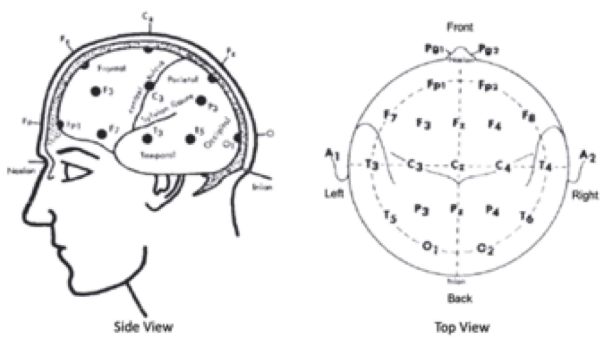
Fig. 7.34. The standard 10-20 system of electrodes to record the EEG.

Why is this placement of electrodes called the “10-20” system? Consider the path starting at the nasion (between the eyes, just above the bridge of the nose), passing over the top of the head, and ending at the inion (a small protuberance at the lower back of the skull). This path is shown as the vertical dashed line in the top view of the head in Fig. 7.34. Five electrodes (O_z, P_z, C_z, F_z, and F_pz) are placed 10, 20, 20, 20, 20, and 10% of the distance along the path. All those 10s and 20s give rise to the name “10-20 system.” The electrodes O_z and F_pz aren’t part of the 10-20 system, so they’re not shown in Fig. 7.34, but their positions are used to properly place the other electrodes.

Now, consider the path starting just behind the left ear (auricle, A₁, sometimes known as the mastoid), passing over the top of the head through C_z, and ending just behind the right ear (A₂); the horizontal dashed line in Fig. 7.34. Five electrodes (T₃, C₃, C_z, C₄, and T₄) are placed 10, 20, 20, 20, 20, and 10% of the distance along the path.

Next, examine the dashed circle in Fig. 7.34, which represents a circumference of the head through O_z, T₃, F_pz, and T₄. Ten electrodes (O₁, T₅, T₃, F₇, F_p1, F_p2, F₈, T₄, T₆, and O₂) are equally spaced along this circumference, each 10% of the way around the circle.

Finally, consider a great circle path passing from F_p1 through C₃ to O₁. The electrode F₃ is halfway between F_p1 and C₃. Similar reasoning gets you the positions of P₃, F₄ and P₄.

How do these electrodes get their funny names? The first letter indicates the region of the brain: F for frontal (front), T for temporal (side, named for your temples), P for parietal (center-back), O for occipital (lower back), Fp for pre-frontal, and C for central. A subscript z means along the midline. Even numbers are used for the right of the head, and odd numbers for the left.

The 10-20 system was proposed by a committee of the International Federation of Clinical Neurophysiology, in order to standardize EEG recordings among different laboratories. 

Measurement of the 10-20 system of electrodes (part 1).
https://www.youtube.com/watch?v=ciGgCoPpPFY

Measurement of the 10-20 system of electrodes (part 2).

https://www.youtube.com/watch?v=Qd4kIvPOQM8

MRI Safety

Will Morton, a staff writer for AuntMinnie.com, published an article about safety issues during magnetic resonance imaging. It begins

As the push toward stronger and faster MRI scanners continues, so does concern over magnet safety, according to Filiz Yetisir, who discussed the potential effects MRI has on patients at the recent International Society for Magnetic Resonance in Medicine virtual meeting (ISMRM 2021).

Main Magnet

An MRI device creates a magnetic field having a strength of several tesla. Any magnetic objects near the device can be sucked into the main field, becoming dangerous projectiles. For instance, in 2001 a six-year-old was killed by an oxygen cylinder. Yetisir warns: “Remember, the magnet’s always on.”

Gradient Coils

The gradient coils used during imaging produce magnetic fields much weaker than the dc main field, but they are turned on and off throughout the imaging pulse sequence. This causes two safety concerns. 1) The changing magnetic field induces eddy currents in the patient, which can stimulate nerves—an effect similar to transcranial magnetic simulation. 2) The switching of current in the gradient coils creates mechanical vibrations, leading to noise so loud that ear plugs may be needed to prevent hearing loss.

Radiofrequency Fields

A radiofrequency magnetic field—which rotates the spins into the plane perpendicular to the main magnet—is an essential part of any MRI pulse sequence. This field can induce eddy currents that heat the tissue. Generally the field isn’t strong enough to cause significant heating, but if a person has metal implants or tattoos, the heating may be increased locally. Any implanted medical device, such as a pacemaker, can interact with all three types of magnetic fields.

Gadolinium

One issue Morton’s article doesn’t discuss is the toxicity of contrast agents such as gadolinium used in some MRI studies.

AuntMinnie.com is one of those websites that’s valuable for readers of Intermediate Physics for Medicine and Biology.

Screenshot of AuntMinnie.com

AuntMinnie.com provides the first comprehensive community internet site for radiologists and related professionals in the medical imaging industry.

We provide a forum for radiologists, business managers, technologists, members of organized medicine, and industry to meet, transact, research, and collaborate on topics within the field of radiology with the ease and speed that only the internet can provide.

AuntMinnie features the latest news and information about medical imaging. Staff members include executives, editors, and software engineers with years of experience in the radiology industry.

AuntMinnie.com reminds me of the Physicsworld medical physics website. Physicsworld is associated with the Institute of Physics, the main physics professional society in the United Kingdom. AuntMinnie is run by a consulting firm, the Science and Medicine Group of Arlington, Virginia. Both websites provide useful information about innovations and news in medical physics. 

Screenshot of MRISafety.com

For more information about MRI safety, see MRIsafety.com. For more information about the physics underlying these safety issues, see Chapter 18 of IPMB.

Photodynamic Therapy

In Chapter 14 of Intermediate Physics for Medicine and Biology, Russ Hobbie and I discuss photodynamic therapy.

Photodynamic therapy (PDT) uses a drug called a photosensitizer that is activated by light (Zhu and Finlay 2008; Wilson and Patterson 2008). PDT can treat accessible solid tumors such as basal cell carcinoma, a type of skin cancer (see Sect. 14.10.4). An example of PDT is the surface application of 5-aminolevulinic acid, which is absorbed by the tumor cells and is transformed metabolically into the photosensitizer protoporphyrin IX. When this molecule interacts with light in the 600–800-nm range (red and near infrared), often delivered with a diode laser, it converts molecular oxygen into a highly reactive singlet state that causes necrosis, apoptosis (programmed cell death), or damage to the vasculature that can make the tumor ischemic. Some internal tumors can be treated using light carried by optical fibers introduced through an endoscope.

The photosensitizer molecule interacts with near infrared light to damage tissue, kill cells, and harm blood vessels. A photon of infrared light doesn’t have much energy, and I’m surprised it can trigger all this destruction. What’s the structure of this molecule that causes so much carnage?

Let’s start with 5-aminolevulinic acid, which is an endogenous nonproteinogenic amino acid. By “endogenous” I mean it occurs naturally in the body. It’s part of the biochemical pathway that leads to the production of heme in animals, and chlorophyll in plants. By “amino acid” I mean it has an amine group (-NH₂) on one end and a carboxylic acid group (-COOH) on the other end. The amino acids that make up proteins have a single carbon atom connecting the amine to the carboxylic acid, like in glycine. 5-aminolevulinic acid, on the other hand, has several carbons linking the two groups. By “nonproteinogenic” I mean that this amino acid is not one that is encoded by our genome, and therefore it never occurs in proteins. Below is a drawing of the structure of 5-aminolevulinic acid.

The chemical structure of 5-aminolevulinic acid. From Wikipedia.

Protoporphyrin IX is a complicated molecule that appears in those same pathways leading to heme and chlorophyll. It contains four pyrrole subunits, each of which is a five-membered ring composed of four carbon atoms and one nitrogen atom. It is nearly planar, and has its four nitrogen atoms facing a central hole. I show its structure below. 

The chemical structure of protoporphyrin IX. From Wikipedia.

In heme, an iron atom occupies the central hole, and is where oxygen binds in the protein hemoglobin found in red blood cells. In chlorophyll, a magnesium atom sits in the central hole.

Most molecules (for instance, water, carbon dioxide, methane, ammonia, urea, and glucose) don’t react when exposed to visible or infrared light, but protoporphyrin IX does. It’s closely related to chlorophyll, which is a key molecule in photosynthesis. When sunlight interacts with chlorophyll, it triggers a series of chemical reactions that leads to the production of carbohydrates from water and carbon dioxide.

I guess I’m not so surprised after all that protoporphyrin IX can wreak so much havoc when exposed to light.

Electroporation

In Chapter 9 of Intermediate Physics for Medicine and Biology, Russ Hobbie and I mention electroporation.

Electrical burns, cardiac pacing, and nerve and muscle stimulation are produced by electric or rapidly changing magnetic fields. Even stronger electric fields increase membrane permeability. This is believed to be due to the transient formation of pores (electroporation). Pores can be formed, for example, by microsecond-length pulses with a field strength in the membrane of about 10⁸ V m⁻¹ (Weaver 2000).

Weaver (2000)
IEEE Trans Plasma Sci,
28: 24–33.

The citation is to an article by James Weaver

Weaver, J. C. (2000) “Electroporation of Cells and Tissues,” IEEE Transactions on Plasma Science, Volume 28, Pages 24–33.

The abstract to the paper is given below.

Electrical pulses that cause the transmembrane voltage of fluid lipid bilayer membranes to reach at least U_m ≈ 0.2 V, usually 0.5–1 V, are hypothesized to create primary membrane “pores” with a minimum radius of ~1 nm. Transport of small ions such as Na⁺ and Cl⁻ through a dynamic pore population discharges the membrane even while an external pulse tends to increase U_m, leading to dramatic electrical behavior. Molecular transport through primary pores and pores enlarged by secondary processes provides the basis for transporting molecules into and out of biological cells. Cell electroporation in vitro is used mainly for transfection by DNA introduction, but many other interventions are possible, including microbial killing. Ex vivo electroporation provides manipulation of cells that are reintroduced into the body to provide therapy. In vivo electroporation of tissues enhances molecular transport through tissues and into their constituative cells. Tissue electroporation, by longer, large pulses, is involved in electrocution injury. Tissue electroporation by shorter, smaller pulses is under investigation for biomedical engineering applications of medical therapy aimed at cancer treatment, gene therapy, and transdermal drug delivery. The latter involves a complex barrier containing both high electrical resistance, multilamellar lipid bilayer membranes and a tough, electrically invisible protein matrix.

Electroporation occurs for transmembrane potentials of a few hundred millivolts, which is only a few times the normal resting potential. I find it amazing that normal resting cells can are so precariously close to electroporating spontaneously. 

One of the most interesting uses of electroporation is transfection: the process of introducing DNA into a cell using a method other than viral infection. This could be used in an experiment in which DNA for a particular gene is transfected into many host cells. If an electric shock is not too violent, the pores created during electroporation will close over several seconds, allowing the cell to then continue its normal function while containing a foreign strand of DNA.

During defibrillation of the heart, the shock can be strong enough to damage or kill cardiac cells. One mechanism for cell injury during electrocution is electroporation followed by entry of extracellular ions such as Ca⁺⁺ that can kill a cell. This raises the possibility of using electroporation to treat cancer by irreversibly killing tumor cells.

Electroporation-based technologies and treatments. https://www.youtube.com/watch?v=u8IeoTg_wTE

Albumin

The structure of albumin. Created by Jawahar Swaminathan and MSD staff at the European Bioinformatics Institute, on Wikipedia.

A physicist working in medicine or biology needs to know some biochemistry. Not much, but enough to understand the structure and function of the most important biological molecules. For instance, one type of molecule that plays a key role in biology is protein. In the first section of Chapter 1 in Intermediate Physics for Medicine and Biology, Russ Hobbie and I write

Proteins are large, complex macromolecules that are vitally important for life. For example, hemoglobin is the protein in red blood cells that binds to and carries oxygen. Hemoglobin is roughly spherical, about 6 nm in diameter.

While hemoglobin is one of the most well-known and important proteins, in this post I’d like to introduce proteins using a different example: albumin. To be precise, human serum albumin. It’s nearly the same size and weight as hemoglobin, and both are found in the blood; hemoglobin in the red blood cells, and albumin in the plasma. Both are globular proteins, meaning they have a roughly spherical shape and are somewhat water soluble. Also, they are both transport proteins: hemoglobin transports oxygen, and albumin transports a variety of molecules including fatty acids and thyroid hormones.

Albumin is mentioned in Chapter 5 of IPMB because it’s the most abundant protein in blood serum, and therefore is important in determining the osmotic pressure of blood. It appears in a terrifying story told in Homework Problem 7 of Chapter 5, dealing with a hospital pharmacy that improperly dilutes a 25% solution of albumin with pure water instead of saline, causing a patient to go into renal failure. It’s also discussed in Chapter 17 of IPMB, where aggregated albumin microspheres are tagged with technetium-99m and used for nuclear medicine imaging.

All proteins are strings, or polymers, of amino acids. There are 21 amino acids commonly found in proteins. Each one has a different side chain. An amino acid is often denoted by a one-letter code. For example, G is glycine, R is arginine, and H is histidine. 

The amino acids. Created by Dancojocari on Wikopedia.

The primary structure of a protein is simply a list of its amino acids in order. Below is the primary structure of albumin.

MKWVTFISLLFLFSSAYSRGVFRRDAHKSEVAHRFKDLGEENFKALVLIAFAQYLQQCPFEDHVKLVNEVTEFAKTCVADESAENCDKSLHTLFGDKLCTVATLRETYGEMADCCAKQEPERNECFLQHKDDNPNLPRLVRPEVDVMCTAFHDNEETFLKKYLYEIARRHPYFYAPELLFFAKRYKAAFTECCQAADKAACLLPKLDELRDEGKASSAKQRLKCASLQKFGERAFKAWAVARLSQRFPKAEFAEVSKLVTDLTKVHTECCHGDLLECADDRADLAKYICENQDSISSKLKECCEKPLLEKSHCIAEVENDEMPADLPSLAADFVESKDVCKNYAEAKDVFLGMFLYEYARRHPDYSVVLLLRLAKTYETTLEKCCAAADPHECYAKVFDEFKPLVEEPQNLIKQNCELFEQLGEYKFQNALLVRYTKKVPQVSTPTLVEVSRNLGKVGSKCCKHPEAKRMPCAEDYLSVVLNQLCVLHEK

Amino acid polymers often fold into secondary structures. The most common is the alpha helix, held together by hydrogen bonds between hydrogen and nitrogen atoms in nearby amino acids. 

The tertiary structure refers to how the entire amino acid string folds up into its final shape. At the top of this post is a picture of the tertiary structure of albumin. You can see many red alpha helices. 

A mutation is when one or more of the amino acids is replaced by an incorrect one. For instance, in familial dysalbuminemic hyperthyroxinemia, one arginine amino acid is replaced by histidine, which affects how albumin interacts with the thyroid hormones.

Albumin is made in your liver, and a serum albumin blood test can assess liver function. Section 5.4.2 of IPMB discusses some illnesses caused by incorrect osmotic pressure of the blood, which are often associated with abnormal albumin concentrations.

5.4.2 Nephrotic Syndrome, Liver Disease, and Ascites

Patients can develop an abnormally low amount of protein in the blood serum, hypoproteinemia, which reduces the osmotic pressure of the blood. This can happen, for example, in nephrotic syndrome. The nephrons (the basic functioning units in the kidney) become permeable to protein, which is then lost in the urine. The lowering of the osmotic pressure in the blood means that the [driving pressure] rises. Therefore, there is a net movement of water into the interstitial fluid. Edema can result from hypoproteinemia from other causes, such as liver disease and malnutrition.

A patient with liver disease may suffer a collection of fluid in the abdomen. The veins of the abdomen flow through the liver before returning to the heart. This allows nutrients absorbed from the gut to be processed immediately and efficiently by the liver. Liver disease may not only decrease the plasma protein concentration, but the vessels going through the liver may become blocked, thereby raising the capillary pressure throughout the abdomen and especially in the liver. A migration of fluid out of the capillaries results. The surface of the liver “weeps” fluid into the abdomen. The excess abdominal fluid is called ascites.

Albumin is such a common, everyday protein that bovine serum albumin, from cows, is often used in laboratory experiments when a generic protein is required.

The Bystander Effect and a Supralinear Dose-Response Curve

When discussing the biological effects of radiation in Intermediate Physics for Medicine and Biology, Russ Hobbie and I describe the bystander effect. 

Ionization damage is not the entire story. The bystander effect in radiobiology refers to the “induction of biological effects in cells that are not directly traversed by a charged particle, but are in close proximity to cells that are” (Hall 2003; Hall and Giaccia 2012).

Hall (2003) “The Bystander Effect,”
Health Physics, 85:31–35.

I sometimes reread the references we cite, looking for interesting tidbits to share in this blog. Below is the abstract to the 2003 article by Eric Hall about the bystander effect (Health Physics, Vol. 85, Pages 31–35).

The bystander effect refers to the induction of biological effects in cells that are not directly traversed by a charged particle. The data available concerning the bystander effect fall into two quite separate categories, and it is not certain that the two groups of experiments are addressing the same phenomenon. First, there are experiments involving the transfer of medium from irradiated cells, which results in a biological effect in unirradiated cells. Second, there is the use of sophisticated single particle microbeams, which allow specific cells to be irradiated and biological effects studied in their neighbors; in this case communication is by gap junction. Medium transfer experiments have shown a bystander effect for cell lethality, chromosomal aberrations and cell cycle delay. The type of cell, epithelial vs. fibroblast, appears to be important. Experiments suggest that the effect is due to a molecule secreted by irradiated cells, which is capable of transferring damage to distant cells. Use of a single microbeam has allowed the demonstration of a bystander effect for chromosomal aberrations, cell lethality, mutation, and oncogenic transformation. When cells are in close contact, allowing gap junction communication, the bystander effect is a much larger magnitude than the phenomenon demonstrated in medium transfer experiments. A bystander effect has been demonstrated for both high- and low-LET radiations but it is usually larger for densely ionizing radiation such as alpha particles. Experiments have not yet been devised to demonstrate a comparable bystander effect on a three-dimensional normal tissue. Bystander studies imply that the target for the biological effects of radiation is larger than the cell and this could make a simple linear extrapolation of radiation risks from high to low doses of questionable validity.

Our discussion of the bystander effect in IPMB closely parallels that given by Hall. But in his article Hall wrote this

This bystander effect can be induced by radiation doses as low as 0.25 mGy and is not significantly increased up to doses of 10 Gy

and this

When 10% of the cells on a dish are exposed to two or more alpha particles, the resulting frequency of induced oncogenic transformation is indistinguishable from that when all the cells on the dish are exposed to the same number of alpha particles.

What?!? The bystander effect is not increased when the dose increases by a factor of forty thousand? You can fire three alpha particles per cell at only one out of every ten cells and the response is the same as if you fire three alpha particles per cell at every cell? I don’t understand. 

Another surprising feature of the data is that all these changes are different than they are for zero dose. That means the dose-response curve must start at zero, jump up to a significant level, and then be nearly flat. Such a dose-response behavior is different than that predicted by the linear no-threshold model (linearly extrapolating from what is known about radiation risk at high doses down to low doses). Indeed, that is what Hall is hinting at in the last sentence of his abstract.

Below is a slightly modified version of Figure 16.51 from IPMB. It shows different assumptions for how tissue responds to a dose of radiation. Data exists (the data points with error bars) for moderate doses, but what happens at very low doses? The standard dogma is the linear no-threshold model (LNT), which is a linear extrapolation from the data at moderate doses down to zero. Some believe there is a threshold below which low doses of radiation have no effect, and a few researchers even claim that very low doses can be beneficial (hormesis). Hall’s hypothesis is that the bystander effect would have a larger impact at low doses than predicted by the linear no-threshold model. It would be a supralinear effect. Based on Fig. 6 of Hall’s article, the effect would be dramatic, like the red bystander curve I added to our figure below. 

Possible responses of tissue to various doses of radiation. The two lowest-dose
measurements are shown. With zero dose there is no excess effect.
Adapted from Fig. 16.51 of Intermediate Physics for Medicine and Biology.

Previously in this blog, I have expressed skepticism of the linear no-threshold model, leaning more toward a threshold model in which very low doses have little or no effect. Hall’s claim implies the opposite: very low doses would have a bigger effect than expected from the linear no-threshold model. What do I make of this? First, let me say that I’m speculating in a field that’s outside my area of expertise; I’m not a radiation biologist. But to me, it seems odd to say that zapping 10% of the cells with alpha particles will have the same effect as zapping 100% of the cells with alpha particles. And it sounds strange to say that the response is not significantly affected by increasing the dose by a factor of 40,000. I don't usually ask for assistance from my readers, but if anyone out there has an explanation for how this dramatic supralinear effect works, I would appreciate hearing it. 

One of the most important questions raised in IPMB is: What is the true risk from low doses of radiation. The bystander effect is one factor that goes into answering this question. We need to understand it better.

The career of Eric Hall. https://www.youtube.com/watch?v=eh6erz_Ds0M

 

Klein-Nishina Formula for Polarized Photons

In Chapter 15 of Intermediate Physics for Medicine and Biology, Russ Hobbie and I discuss Compton Scattering. An incident photon scatters off a free electron, producing a scattered photon and a recoiling electron. We write

The inclusion of dynamics, which allows us to determine the relative number of photons scattered at each angle, is fairly complicated. The quantum-mechanical result is known as the Klein-Nishina formula (Attix 1986). The result depends on the polarization of the photons. For unpolarized photons, the cross section per unit solid angle for a photon to be scattered at angle θ is

 

where

is the classical radius of the electron. [The variable x is the ratio of the incident photon’s energy to the rest energy of the electron.]

What happens for polarized photons? In that case, the scattering may depend on the angle φ with respect to the direction of the electric field. The resulting scattering formula is

Unpolarized light means that you average over all angles φ, implying that factors of cos²φ become ½. A bit of algebra should convince you that when the expression above is averaged over φ it’s equivalent to Eq. 15.16 in IPMB.

In order to analyze polarized photons, we must consider the two polarization states, φ = 0 and φ = 90°.

φ = 0

The incident and scattered photon directions define a plane. Assume the electric field associated with the incident photon lies in this plane, as shown in the drawing below. From a classical point of view, the electric field will cause the electron to oscillate, resulting in dipole radiation (a process called Thomson scattering). A dipole radiates perpendicular to its direction of oscillation, but not parallel to it. Therefore, you get scattering for θ = 0 and 180°, but not for θ = 90°.

A schematic diagram of Compton scattering for polarized light with φ = 0.

A quantum-mechanical analysis of this behavior (Compton scattering) accounts for the momentum of the incident photon and the recoil of the electron. In the quantum case, some scattering occurs at θ = 90°, but it is suppressed unless the energy of the incident photon is much greater than the rest mass of the electron (x >> 1).

φ = 90°

For Thomson scattering, if the electric field oscillates perpendicular to the scattering plane (shown below) then all angles θ are perpendicular to the dipole and therefore should radiate equally. This effect is also evident in a quantum analysis unless x >> 1.

A schematic diagram of Compton scattering for polarized light with φ = 90°.

The figure below is similar to Fig. 15.6 in IPMB. The thick, solid lines indicate the amount of scattering (the differential cross section) for unpolarized light, as functions of θ. The thin dashed curves show the scattering for φ = 0 and the thin dash-dot curves show it for φ = 90°. The red curves are for a 10 keV photon, whose energy is much less than the 511 keV rest energy of an electron (x << 1). The behavior is close to that of Thomson scattering. The light blue curves are for a 1 GeV photon (1,000,000 keV). For such a high energy (x >> 1) almost all the energy goes to the recoiling electron, with little to the scattered photon. The dashed and dash-dot curves are present, but they overlap with the solid curve and are not distinguishable from it. Polarization makes little difference at high energies. 

The differential cross section for Compton scattering. The incident photon energy for each curve is shown on the right. The solid curves are for unpolarized light, the dashed curves are for light with φ = 0, and the dash-dot curves are for φ = 90°. Adapted from Fig. 15.6 in IPMB.

Why is there so little backscattering (θ = 180°) for high energy photons? It’s because the photon has too much momentum to have its direction reversed by a light electron. It would be like a truck colliding with a mosquito, and after the collision the truck recoils backwards. That’s extraordinarily unlikely. We all know what will happen: the truck will barrel on through with little change to its direction. Any scattering occurs at small angles. 

 

Notice that Thomson scattering treats light as a wave and predicts what an oscillating electric field will do to an electron. Compton scattering treats light as a photon having energy and momentum, which interacts with an electron like two colliding billiard balls. That is wave-particle duality, and is at the heart of a quantum view of the world. Who says IPMB doesn’t do quantum mechanics?

Is Shot Noise Also White Noise?

In Chapters 9 and 11 of Intermediate Physics for Medicine and Biology, Russ Hobbie and I discuss shot noise.

9.8.1 Shot Noise

The first (and smallest) limitation [on our ability to measure current] is called shot noise. It is due to the fact that the charge is transported by ions that move randomly and independently through the channels....

11.16.2 Shot Noise

Chapter 9 also mentioned shot noise, which occurs because the charge carriers have a finite charge, so the number of them passing a given point in a circuit in a given time fluctuates about an average value. One can show that shot noise is also white noise [my italics].

Introduction to Membrane Noise,
by Louis DeFelice

How does one show that shot noise is white noise (independent of frequency)? I’m going to follow Lou DeFelice’s explanation in his book Introduction to Membrane Noise (cited in IPMB). I won’t give a rigorous proof. Instead, I’ll first state Campbell’s theorem (without proving it), and then show that the whiteness of shot noise is a consequence of that theorem.

Campbell’s Theorem

To start, I’ll quote DeFelice, but I will change the names of a few variables.

Suppose N impulses i(t) arrive randomly in the time interval T. The sum of these will result in a random noise signal I(t). This is shown qualitatively in Figure 78.1.

Below is my version of Fig. 78.1.

A diagram illustrating the sum of N impulses, i(t), each shown in red, arriving randomly in the time interval T. The blue curve represents their sum, I(t), and the green dashed line represents the average, <I(t)>. Adapted from Fig. 78.1 in Introduction to Membrane Noise by Louis DeFelice.

DeFelice shows that the average of I(t), which I’ll denote <I(t)>, is

Here he lets T and N both be large, but their ratio (the average rate that the impulses arrived) remains finite.

He then shows that the variance of I(t), called σ_I², is

Finally, he writes

In order to calculate the spectral density of I(t) from i(t) we need Rayleigh’s theorem [also known as Parseval’s theorem]…

where î(f) is the Fourier transform of i(t) [and f is the frequency].

He concludes that the spectral density S_I(f) is given by

These three results (for the average, the variance, and the spectral density) constitute Campbell’s theorem.

Shot Noise

Now, let’s analyze shot noise by using Campbell’s theorem assuming the impulse is a delta function (zero everywhere except at t = 0 where it’s infinite). Set i(t) = q δ(t), where q is the charge of each discrete charge carrier.

First, the average <I(t)> is simply Nq/T, or the total charge divided by the total time. 

Second, the variance is the integral of the delta function squared. When any function is multiplied by a delta function and then integrated over time, you get that function evaluated at time zero. So, the integral of the square of the delta function gives the delta function itself evaluated at zero, which is infinity. Yikes! The variance of shot noise is infinite.

Third, to get the spectral density of shot noise we need the Fourier transform of the delta function. 

The key point is that S_I(f) is independent of frequency; it’s white.

DeFelice ends with

This [the expression for the spectral density] is the formula for shot noise first derived by Schottky (1918, pp. 541-567) in 1918. Evidently, the variance defined as

is again infinite; this is a consequence of the infinitely small width of the delta function.

As DeFelice reminds us, shot noise is white because the delta function is infinitely narrow. As soon as you assume i(t) has some width (perhaps the time it takes for a charge to cross the membrane), the spectrum will fall off at high frequencies, the variance won’t be infinite (thank goodness!), and the noise won’t be white. The bottom line is that shot noise is white because the Fourier transform of a delta function is a constant.

Conclusion

Perhaps you’re thinking I haven’t helped you all that much. I merely changed your question from “why is shot noise white” to “how do I prove Campbell’s theorem.” You have a point. Maybe proving Campbell’s theorem can be the story of another post.

I met Lou DeFelice in 1984, when I was a graduate student at Vanderbilt University and he came to give a talk. In the summer of 1986, my PhD advisor John Wikswo and I traveled to Emory University to visit DeFelice and Robert DeHaan. During that trip, Wikswo and I were walking across the Emory campus when Wikswo decided he knew a short cut (he didn’t). He left the sidewalk and entered a forest, with me following behind him. After what seemed like half an hour of wandering through a thicket, we emerged from the woods at a back entrance to the Yerkes Primate Research Center. We’re lucky we weren’t arrested.

DeFelice joined the faculty at Vanderbilt in 1995, and we both worked there in the late 1990s. He was a physicist by training, but spent most of his career studying electrophysiology. Sadly, in 2016 he passed away.

The Unit of Vascular Resistance: A Naming Opportunity

The metric system is based on three fundamental units: the kilogram (kg, mass), the meter (m, distance), and the second (s, time). Often a combination of these three is given a name (called a derived unit), usually honoring a famous scientist. For example, a newton, the unit of force named after the English physicist and mathematician Isaac Newton (1642 – 1727), is a kg m s⁻²; a joule, the unit of energy named for English physicist James Joule (1818 – 1889), is a kg m² s⁻²; a pascal, the unit of pressure named for French mathematician and physicist Blaise Pascal (1623 – 1662), is a kg m⁻¹ s⁻²; a watt, the unit of power named for Scottish engineer James Watt (1736 – 1819), is a kg m² s⁻³; and a rayl, the unit of acoustic impedance named for English physicist John Strutt (1842 – 1919) who is also known as Lord Rayleigh, is a kg m⁻² s⁻¹.

In Chapter 1 of Intermediate Physics for Medicine and Biology, Russ Hobbie and I discuss the human circulatory system. We talk about blood pressure, p, which is usually expressed in mmHg or torr, but in the metric system is given in pascals. We also analyze blood flow or cardiac output, i, sometimes expressed in milliliters per minute, but properly should be m³ s⁻¹. Then Russ and I introduce is the vascular resistance.

We define the vascular resistance R in a pipe or a segment of the circulatory system as the ratio of pressure difference across the pipe or segment to the flow through it:

R = Δp/i .                  (1.58)

The units are Pa m⁻³ s. Physiologists use the peripheral resistance unit (PRU), which is torr ml⁻¹ min.

What name is given to the Pa m⁻³ s, or equivalently the kg m⁻⁴ s⁻¹? Sometimes it’s called the “acoustic ohm,” stressing its analogy to the electrical unit of the ohm (a volt per amp). If the unit for electrical resistance can honor a scientist, German physicist Georg Ohm (1789 – 1854), why can’t the unit for mechanical resistance do the same? Let’s name the unit for vascular resistance!

I know what you’re thinking: we already have a name, the peripheral resistance unit. True, but I see three disadvantages with the PRU. First, it’s based on oddball units (pressure in torr? time in minutes?), so it’s not standard metric. Second, sometimes it’s defined using the second rather than the minute, so it’s confusing and you always must be on your toes to avoid making a mistake. Third, it wastes the chance to honor a scientist. We can do better.

My first inclination was to name this unit after the French physician Jean Poiseuille (1797 – 1869). He is the hero of Sec. 1.17 in IPMB. His equation relating the pressure drop and flow through a tube—often called the Poiseuille law—explains much about blood flow. However, Poiseuille already has a unit. The coefficient of dynamic viscosity has units of kg m⁻¹ s⁻¹, which is sometimes called a poiseuille. It’s not used much, but it would be confusing to adopt it for vascular resistance in addition to viscosity. Moreover, the old cgs unit for viscosity, g cm⁻¹ s⁻¹, is also named for Poiseuille; it’s called the poise, and it is commonly used. With two units already, Poiseuille is out.

Henry Darcy (1803 – 1858) was a French engineer who made important contributions to hydraulics, including Darcy’s law for flow in a porous medium. However, an older unit of hydraulic permeability is the darcy. Having another unit named after Darcy (even if it’s an mks unit instead of an oddball obsolete unit) would complicate things. So, no to Mr. Darcy.

The Irish physicist and mathematician George Stokes (1819 – 1903) helped develop the theoretical justification for the Poiseuille law. I’m a big fan of Stokes. He seems like a perfect candidate. However, the cgs unit of kinematic viscosity, the cm² s⁻¹, is called the stokes. He’s taken.

The Poiseuille law is sometimes called the Hagen-Poiseuille law, after the German scientist Gotthilf Hagen (1797 – 1884). He would be a good candidate for the unit, and some might choose to call a kg m⁻⁴ s⁻¹ a hagen. Why am I not satisfied with this choice? Hagen appears to be more of a hydraulic engineer than a biomedical scientist, and one theme in IPMB is to celebrate researchers who work at the interface between physics and physiology. Nope.

A portrait of William Harvey,
downloaded from wikipedia
(public domain).

My vote goes to William Harvey (1578 – 1657), the English physician who first discovered the circulation of blood. I can find no units already named for Harvey. He doesn’t have a physics education, but he did make quantitative estimates of blood flow to help establish his hypothesis of blood circulation (such numerical calculations were uncommon in his day, but are in the spirit of IPMB). Harvey is a lot easier to pronounce than Poiseuille. Moreover, my favorite movie is Harvey.

We can name the kg m⁻⁴ s⁻¹ as the harvey (Ha), and 1 Ha = 1.25 × 10^-10 PRU (we may end up using gigaharveys when analyzing the peripheral resistance in people). One final advantage of the harvey: for those of you who disagree with me, you can claim that “Ha" actually stands for Hagen.

Ceaseless Motion: William Harvey’s Experiments in Circulation.

https://www.youtube.com/watch?v=w6q50_qNMoA

 

The trailer from the 1950 film Harvey,

starring James Stewart as Elwood P. Dowd.

https://www.youtube.com/watch?v=VvfXvW2wsuQ

Can Induced Electric Fields Explain Biological Effects of Power-Line Magnetic Fields?

Sometimes proponents of pseudoscience embrace nonsense, but other times they propose plausible-sounding ideas that are wrong because the numbers don’t add up. For example, suppose you are discussing with your friend about the biological effects of power-line magnetic fields. Your friend might say something like this:

“You keep claiming that magnetic fields don’t have any biological effects. But suppose it’s not the magnetic field itself, but the electric field induced by the changing magnetic field that causes the effect. We know an electric field can stimulate nerves. Perhaps power-line effects operate like transcranial magnetic stimulation, by inducing electric fields.”

Well, there’s nothing absurd about this hypothesis. Transcranial magnetic stimulation does work by creating electric fields in the body via electromagnetic induction, and these electric fields can stimulate nerves. The qualitative idea is reasonable. But does it work quantitatively? If you do the calculation, the answer is no. The electric field induced by a power line is less than the endogenous electric field associated with the electrocardiogram. You don’t have to perform a difficult, detailed calculation to show this. A back-of-the-envelope estimation suffices. Below is a new homework problem showing you how to make such an estimate.

Section 9.10

Problem 36 ½. Estimate the electric field induced in the body by a power-line magnetic field, and compare it to the endogenous electric field in the body associated with the electrocardiogram.

(a) Use Eq. 8.25 to estimate the induced electric field, E. The magnetic field in the vicinity of a power line can be as strong as 5 μT (Possible Health Effects of Exposure to Residential Electric and Magnetic Fields, 1997, Page 32), and it oscillates at 60 Hz. The radius, a, of the current loop in our body is difficult to estimate, but take it as fairly large (say, half a meter) to ensure you do not underestimate the induced electric field.

(b) Estimate the endogenous electric field in the torso from the electrocardiogram, using Figures 7.19 and 7.23.

(c) Compare the electric fields found in parts (a) and (b). Which is larger? Explain how an induced electric field could have an effect if it is smaller than the electric fields already existing in the body.

Let’s go through the solution to this new problem. First, part (a). The amplitude of the magnetic field is 0.000005 T. The field oscillates with a period of 1/60 Hz, or about 0.017 s. The peak rate of change will occur during only a fraction of this period, and a reasonable approximation is to divide the period by 2π, so the time over which the magnetic field changes is 0.0027 s. Thus, the rate of change dB/dt is 0.000005 T/0.0027 s, or about 0.002 T/s. Now use Eq. 8.25, E = a/2 dB/dt (ignore the minus sign in the equation, which merely indicates the phase), with a = 0.5 m, to get E = 0.0005 V/m.

Now part (b). Figure 7.23 indicates that the QRS complex in the electrocardiogram has a magnitude of about ΔV = 0.001 V (one millivolt). Figure 7.19 shows that the distance between leads is on the order of Δr = 0.5 m. The magnitude of the electric field is approximately ΔV/Δr = 0.002 V/m.

In part (c) you compare the electric field induced by a power line, 0.0005 V/m, to the electric field in the body caused by the electrocardiogram, 0.002 V/m. The field produced by the ECG is four times larger. So, how can the induced electric field have a biological effect if we are constantly exposed to larger electric fields produced by our own body? I don’t know. It seems to me that would be difficult.

Hart and Gandhi (1998)
Phys. Med. Biol.,
43:3083–3099.

But wait! Our calculation in part (b) is really rough. Perhaps we should do a more detailed calculation. Rodney Hart and Om Gandhi did just that (“Comparison of cardiac-induced endogenous fields and power frequency induced exogenous fields in an anatomical model of the human body,”  Physics in Medicine & Biology, Volume 43, Pages 3083–3099, 1998). They found that during the QRS complex the endogenous electric field varied throughout the body, but it is usually larger than what we estimated. It’s giant in the heart itself, about 3 V/m. All through the torso it’s more than ten times what we found; for instance, in the intestines it’s 0.04 V/m. Even in the brain the field strength (0.014 V/m) is seven times larger than our estimate (0.002 V/m).

Moreover, the heart isn’t the only source of endogenous fields (although it’s the strongest). The brain, peripheral nerves, skeletal muscle, and the gut all produce electric fields. In addition, our calculation of the induced electric field is evaluated at the edge of the body, where the current loop is largest. Deeper within the torso, the field will be less. Finally, our value of 5 μT is extreme. Magnetic fields associated with power lines are usually about one tenth of this. In other words, in all our estimates we took values that favor the induced electric field over the endogenous electric field, and the endogenous electric field is still four times larger.

What do we conclude? The qualitative mechanism proposed by your friend is not ridiculous, but it doesn’t work when you do the calculation. The induced electric field would be swamped by the endogenous electric field.

The moral of the story is that proposed mechanisms must work both qualitatively and quantitatively. Doing the math is not an optional step to refine your hypothesis and make it more precise. You have to do at least an approximate calculation to decide if your idea is reasonable. That’s why Russ Hobbie and I emphasize solving toy problems and estimation in Intermediate Physics for Medicine and Biology. Without estimating how big effects are, you may go around saying things that sound reasonable but just aren’t true.