|
| Fig. 17.2 in Intermediate Physics for Medicine and Biology. |
 |
| Figure 17.2, with part of the drawing magnified. |
Let’s begin by magnifying the bottom left corner, corresponding to the lightest nuclei. The most abundant isotope of hydrogen consists of a single proton. In general, an isotope is denoted using the chemical symbol with a left subscript Z and a left superscript A. The chemical symbol and atomic number are redundant, so we’ll drop the subscript. A proton is written as 1H.
The nucleus to the right of 1H is 2H, called a deuteron, consisting of one proton and one neutron. Deuterium exists in nature but is rare. The isotope 3H also exists but isn’t stable (its half life is 12 years) so it’s not included in the drawing.
The row above hydrogen is helium, with two stable isotopes: 3He and 4He. You probably know the nucleus 4He by another name; the alpha particle. As you move up to higher rows you find the elements lithium, beryllium, and boron (10B is used for boron neutron capture therapy). Light isotopes tend to cluster around the dashed line Z = N.
 |
| Figure 17.2, with part of the drawing magnified. |
Moving up and to the right brings us to essential elements for life: carbon, nitrogen, and oxygen. Certain values of Z and N, called magic numbers, lead to particularly stable nuclei: 2, 8, 20, 28, 50, 82, and 126. Oxygen is element eight, and Z = 8 is magic, so it has three stable isotopes. The isotope 16O is doubly magic (Z = 8 and N = 8) and is therefore the most abundant isotope of oxygen.
 |
| Figure 17.2, with part of the drawing magnified. |
The next drawing shows the region around 40Ca, which is also doubly magic (Z = 20, N = 20). It is the heaviest isotope having Z = N. Heavier isotopes need extra neutrons to overcome the Coulomb repulsion of the protons, so the region of stable isotopes bends down as it moves right. The dashed line indicating Z = N won’t appear in later figures; it’ll be way left of the magnified region. Four stable isotopes (37Cl, 38Ar, 39K, and 40Ca) have a magic number of neutrons N = 20. Calcium, with its magic number of protons, has five stable isotopes.
No stable isotopes correspond to N = 19 or 21. In general, you’ll find more stable isotopes with even values of Z and N than odd.
 |
| Figure 17.2, with part of the drawing magnified. |
Next we move up to the region ranging from Z = 42 (molybdenum) to Z = 44 (ruthenium). No stable isotopes exist for Z = 43 (technetium); a blank row stretches across the region of stability. As discussed in Chapter 17 of IPMB, the unstable 99Mo decays to the metastable state 99mTc (half life = 6 hours), which plays a crucial role in medical imaging.
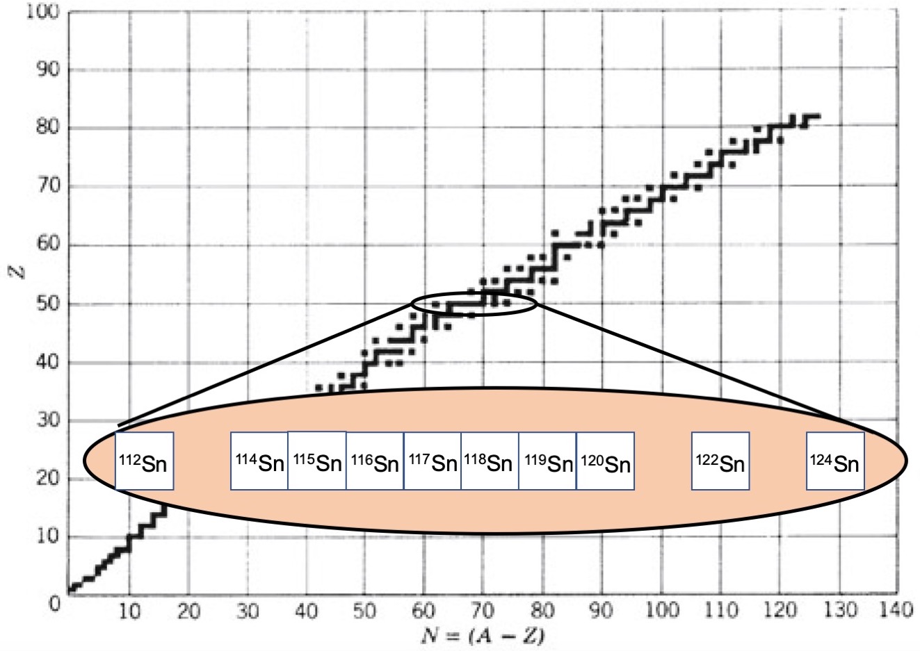 |
| Figure 17.2, with part of the drawing magnified. |
Tin has a magic number of protons (Z = 50), resulting in ten stable isotopes, the most of any element.
 |
| Figure 17.2, with part of the drawing magnified. |
As we move to the right, the region of stability ends. The heaviest stable isotope is lead (Z = 82), which has a magic number of protons and four stable isotopes. Above that, nothing. There are unstable isotopes with long half lives; so long that they are still found on earth. Scientists used to think that an isotope of bismuth, 209Bi (Z = 83, N = 126), was stable, but now we know its half life is 2×10¹⁹ years. Uranium (Z = 92) has two unstable isotopes with half lives similar to the age of the earth, but that’s another story.
If you want to find information about all the stable isotopes, and other isotopes that are unstable, search the web for “table of the isotopes.” Here’s my favorite: https://www-nds.iaea.org/relnsd/vcharthtml/VChartHTML.html.