Friday, October 2, 2020

The Death and Life of the Great Lakes

Many readers of this blog live far from me—sometimes in countries on the other side of the world—and may not be interested in local topics germane to Michigan. Yet the Great Lakes are important to everyone; they hold 20% of the earth’s liquid freshwater. The challenges faced by the Great Lakes aren’t unique; they’re relevant to other watersheds worldwide.

For those who aren’t Michiganders, a drawing of the five Great Lakes looks like a map of Michigan

The Great Lakes
From Phizzy at Wikipedia.

Between its upper and lower peninsulas, Michigan borders four of the five lakes. I live half way between the southern tip of Lake Huron and the western edge of Lake Erie. I’ve visited all five lakes, and I’m concerned about their welfare.
The Death and Life of the Great Lakes,
by Dan Egan.
 
I recently read The Death and Life of the Great Lakes (2017), by Dan Egan. (This book was recommended to me by Congresswoman Elissa Slotkin, who’s now running for reelection in my home district). I’ve lived in Michigan for 22 years, but much of this story was new to me. In his introduction, Egan writes
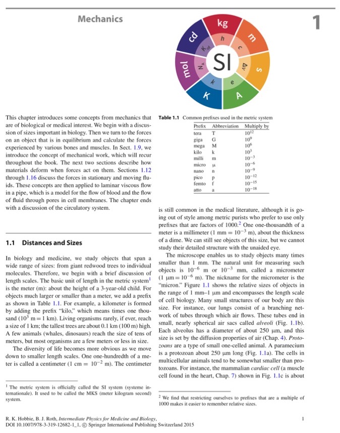
Iconic disasters have a history of prompting government action. Three years after the Cuyahoga River fire of 1969, Congress passed the Clean Water Act. Two decades later, when the Exxon Valdez ran aground and dumped 10.8 million gallons of crude oil into Alaska’s Prince William Sound, images of cleanup crews using paper towels to cleanse tarred birds helped press Congress into doing something it should have done years earlier. It mandated double-hulled oil tankers.

But the disaster unfolding today on the Great Lakes didn’t ignite like a polluted river or gush like oil from a cracked hull, and so far there is no galvanizing image of this slow-motion catastrophe, though a few come to my mind. One is the bow of an overseas ship easing its way into the first navigation lock on the St. Lawrence Seaway, the Great Lakes’ “front door” to fresh waves of biological pollution. Another is a satellite photo of a green-as-paint toxic algae slick smothering as much as 2,000 square miles of Lake Erie.

Yet another is the grotesque mug of an Asian carp, a monster-sized carp imported to the United States in the 1960s and used in government experiments to gobble up excrement in Arkansas sewage lagoons. The fish, which can grow to 70 pounds and eat up to 20 percent of their weight in plankton per day, escaped into the Mississippi River basin decades ago and have been migrating north ever since. There are now mustering at the Great Lakes’ “back door”—the Chicago canal system that created a manmade connection between the previously isolated Great Lakes and the Mississippi basin, which covers about 40 percent of the continental United States. The only thing blocking the fish’s swim through downtown Chicago and into Lake Michigan is an electrical barrier in the canal—one that has a history of unexpected shutdowns.

The Chicago canal has also turned the Great Lakes’ ballast water problem [ships from the Atlantic Ocean having exotic species in their ballast water and then dumping it into the Great Lakes] into a national one, because there are dozens of invasive species poised to ride its waters out of the lakes and into the rivers and water bodies throughout the heart of the continent. Species like the spiny water flea, the threespine stickleback, the bloody red shrimp and the fishhook water flea. All organisms you probably haven’t heard of. Yet.

Few out West, after all, had ever heard of quagga mussels—until they tumbled down the Chicago canal and metastasized across the Mississippi basin and, eventually, into the arid West, likely as hitchhikers aboard recreational boats towed over the Rocky Mountains. The mussels have since unleashed havoc on hydroelectric dams, drinking water systems and irrigation networks in Utah, Nevada and California and the federal government estimates that if the mussels make their way into the Northwest’s Columbia River hydroelectric dam system they could do a half billion dollars of damage—per year.
Much of Egan’s book is about how invasive species interact with native animals. In Chapter 2 of Intermediate Physics for Medicine and Biology, Russ Hobbie and I discuss the predator-prey problem modeled by the Lotka-Volterra equations. It is a useful toy model for understanding the interplay of two species, but it doesn’t explain the workings of a large and complex ecosystem.

The Great Lakes (at least the four that border Michigan) were once isolated from the Atlantic Ocean by Niagara Falls, a barrier than even the most determined fish could not surmount. The opening of the Saint Lawrence Seaway allowed a series of nonnative animals to enter the lakes. First came the sickening sea lamprey that nearly caused the native lake trout to go extinct. Next was an explosion of alewife (a river herring). Scientists introduced coho and Chinook salmon to prey upon the alewives. In each case, the ramifications of a new species were difficult to predict. Then zebra mussels and the quagga muscles arrived, and finally the round goby. It’s a horror story, and I suspect an invasion of the Asian carp is inevitable.

Besides these exotic species, the Great Lakes (especially Lake Erie) suffer from algae blooms triggered by fertilizer runoff. Add in climate change, which is causing the water level in the lakes to fluctuate, and you have an unstable and unhealthy ecosystem. 

I’ll give Egan the last word.
If we can close these doors to future invasions [of invasive species], we may give the lakes, and the rest of the country, time to reach a new equilibrium, a balance between what is left of the natural inhabitants and all the newcomers... And if we do this, then we can focus on the major problems that still plague the lakes, which include the overapplication of farm fertilizer that is helping to trigger the massive toxic algae outbreaks, the impact a warming globe is having on the lake’s increasingly unstable water levels and the need to protect lake waters from outsiders seeking to drain them for their own profit.

Dan Egan on The Death and Life of the Great Lakes at the 2018 L.A. Times Festival of Books. https://www.youtube.com/watch?v=jtq_cN1kPkg


Friday, September 25, 2020

Comparative Anatomy is Largely the Story of the Struggle to Increase Surface in Proportion to Volume

On Being the Right Size, by J. B. S. Haldane, superimposed on Intermediate Physics for Medicine and Biology.
On Being the Right Size,
by J. B. S. Haldane.
J. B. S. Haldane’s essay “On Being the Right Size” is a classic. In the first chapter of Intermediate Physics for Medicine and Biology, Russ Hobbie and I quote it.
You can drop a mouse down a thousand-yard mine shaft; and arriving at the bottom, it gets a slight shock and walks away. A rat is killed, a man is broken, a horse splashes.
Another line from the essay is nearly as famous.
Comparative anatomy is largely the story of the struggle to increase surface in proportion to volume.
We describe the interplay between surface and volume in Chapter 2 of IPMB
Consider the relation of daily food consumption to body mass. This will introduce us to simple scaling arguments. As a first model, we might suppose that each kilogram of tissue has the same metabolic requirement, so that food consumption should be proportional to body mass [or volume]. However, there is a problem with this argument. Most of the food that we consume is converted to heat. The various mechanisms to lose heat—radiation, convection, and perspiration—are all roughly proportional to the surface area of the body rather than its mass.
If ridding our bodies of excess heat is an important issue, then we need to increase surface area without increasing volume. A similar issue arises when getting oxygen to our cells. Our circulatory and respiratory systems are elaborate strategies to increase the area over which oxygen diffuses. This is a key concept where physics and physiology overlap.

You can read Haldane's essay in its entirety here. Below I quote part of it. Enjoy!
Animals of all kinds find difficulties in size for the following reason. A typical small animal, say a microscopic worm or rotifer, has a smooth skin through which all the oxygen it requires can soak in, a straight gut with sufficient surface to absorb its food, and a single kidney. Increase its dimensions tenfold in every direction, and its weight is increased a thousand times, so that if it is to use its muscles as efficiently as its miniature counterpart, it will need a thousand times as much food and oxygen per day and will excrete a thousand times as much of waste products.
Now if its shape is unaltered its surface will be increased only a hundredfold, and ten times as much oxygen must enter per minute through each square millimetre of skin, ten times as much food through each square millimetre of intestine. When a limit is reached to their absorptive powers their surface has to be increased by some special device. For example, a part of the skin may be drawn out into tufts to make gills or pushed in to make lungs, thus increasing the oxygen-absorbing surface in proportion to the animal’s bulk. A man, for example, has a hundred square yards of lung. Similarly, the gut, instead of being smooth and straight, becomes coiled and develops a velvety surface, and other organs increase in complication. The higher animals are not larger than the lower because they are more complicated. They are more complicated because they are larger. Just the same is true of plants. The simplest plants, such as the green algae growing in stagnant water or on the bark of trees, are mere round cells. The higher plants increase their surface by putting out leaves and roots. Comparative anatomy is largely the story of the struggle to increase surface in proportion to volume. Some of the methods of increasing the surface are useful up to a point, but not capable of a very wide adaptation. For example, while vertebrates carry the oxygen from the gills or lungs all over the body in the blood, insects take air directly to every part of their body by tiny blind tubes called tracheae which open to the surface at many different points. Now, although by their breathing movements they can renew the air in the outer part of the tracheal system, the oxygen has to penetrate the finer branches by means of diffusion. Gases can diffuse easily through very small distances, not many times larger than the average length traveled by a gas molecule between collisions with other molecules. But when such vast journeys—from the point of view of a molecule—as a quarter of an inch have to be made, the process becomes slow. So the portions of an insect’s body more than a quarter of an inch from the air would always be short of oxygen. In consequence hardly any insects are much more than half an inch thick. Land crabs are built on the same general plan as insects, but are much clumsier. Yet like ourselves they carry oxygen around in their blood, and are therefore able to grow far larger than any insects. If the insects had hit on a plan for driving air through their tissues instead of letting it soak in, they might well have become as large as lobsters, though other considerations would have prevented them from becoming as large as man.

Friday, September 18, 2020

Spillover: Animal Infections and the Next Human Pandemic

Spillover: Animal Infections and the Next Human Pandemic, by David Quammen, superimposed on Intermediate Physics for Medicine and Biology.
Spillover, by David Quammen
I recently read Spillover: Animal Infections and the Next Human Pandemic, by David Quammen. This book was written eight years ago, but it helped me understand what’s happening today with the coronavirus. Quammen writes:
A person might construe this list [Ebola, HIV, bird flu, West Nile virus, SARS, and now Covid-19] as a sequence of dire but unrelated events—independent misfortunes that have happened to us, to humans, for one unfathomable reason and another. Seen that way, Machupo and the HIVs and SARS and the others are “acts of God” in the figurative (or literal) sense, grievous mishaps of a kind with earthquakes and volcanic eruptions and meteor impacts, which can be lamented and ameliorated but not avoided. That’s a passive, almost stoical way of viewing them. It’s also the wrong way.

Make no mistake, they are connected, these disease outbreaks coming one after another. And they are not simply happening to us; they represent the unintended results of the things we are doing. They reflect the convergence of two forms of crisis on our planet. The first crisis is ecological, the second medical. As the two intersect, their joint consequences appear as a pattern of weird and terrible new diseases, emerging from unexpected sources and raising deep concern, deep foreboding, among the scientists who study them. How do such diseases leap from nonhuman animals into people, and why do they seem to be leaping more frequently in recent years? To put the matter in its starkest form: Human-caused ecological pressures and disruptions are bringing animal pathogens ever more into contact with human populations, while human technology and behavior are spreading those pathogens ever more widely and quickly.
Spillover doesn’t contain much physics, but it does allude to the math describing epidemics, making it relevant to Intermediate Physics for Medicine and Biology. Chapter 3 of Spillover discusses the 1927 model of William Kermack and Anderson McKendrick. I admire Quammen for including the mathematical biology of epidemics in his book, but he seems uncomfortable talking about math, and hesitant about subjecting his readers to it. I’m glad the readers of IPMB don’t place me under the same constraint.

Amid a dense flurry of mathematical manipulations, [Kermack and McKendrick] derived a set of three differential equations describing the three classes of living individuals: the susceptible, the infected, and the recovered. During an epidemic, one class flows into another in a simple schema, SIR, with mortalities falling out of the picture because they no longer belong to the population dynamic. As susceptible individuals become exposed to the disease and infected, as infected individuals either recover (now with immunity) or disappear, the numerical size of each class changes at each moment in time. That’s why Kermack and McKendrick used differential calculus. Although I should have paid better attention to the stuff in high school [I didn’t take calculus until college!], even I can understand (and so can you) that dR/dt = γI merely means that the number of recovered individuals in the population [I would have said “the rate of increase of the number of recovered individuals…”], at a given moment, reflects the number of infected individuals times the average recovery rate.  So much for R, the “recovered” class. The equations for S (“susceptibles”) and I (“infected”) are likewise opaque [not the word I would choose] but sensible. All this became known as an SIR model. It was a handy tool for thinking about infectious outbreaks, still widely used by disease theorists.
Covid-19 is caused by a zoonotic virus: a pathogen that leaps from an animal “reservoir” to infect humans. Quammen focuses on zoonotic viruses in Spillover, but he points out that not all viruses originate in animals. For instance, polio and smallpox are viruses that infect only humans. Once we remove those viruses from the human population, they are gone forever. A zoonotic virus “hides” in some wide animal (bats are a common reservoir) until it makes the jump to humans, so they are extraordinarily difficult to eradicate. Spillover is at its best when it describes these jumps, and the scientists who study them. Moreover, Quammen’s book is an extended case study of the scientific method. Everyone should read it.

Does Quammen predict the Covid-19 pandemic? Sort of. He predicts future pandemics arising from virulent and transmissible viruses that spill over from animal reservoirs. He predicts that our growing population and technology will make such spillovers more common. He even pinpointed coronaviruses as one of the likely suspects that could cause a future plague. What scares me is that Covid-19—as disruptive as it’s been for society—is not virulent enough to be the “Next Big One.” I fear it may be only a hint of things to come.

Worried? Me too. I’ll let Quammen have the final—somewhat hopeful—word [my italics].
I don’t say these things about the ineradicability of zoonoses to render you hopeless and depressed. Nor am I trying to be scary for the sake of scariness. The purpose of this book is not to make you more worried. The purpose of this book is to make you more smart.
 
David Quammen talking about Spillover.

Friday, September 11, 2020

Charlotte's Web

Charlotte's Web, by E. B. White, superimposed on Intermediate Physics for Medicine and Biology.
Charlotte's Web,
by E. B. White

Fern was up at daylight, trying to rid the world of injustice. As a result, she now has a pig.”

        From Charlotte’s Web, by E. B. White


Intermediate Physics for Medicine and Biology never mentions spiders like Charlotte, does it? It does! Chapter 1 has a homework problem about the strength of a spider’s thread. Steven Vogel discusses this in his terrific book Life’s Devices.

Anything with a strength at or above 100 MPa has to be considered a good tensile material—wood with the grain and collagen have about this value. Nylon [1000 MPa] is outstanding… and spider silk [2000 MPa] is superb—one can only wonder why, if one kind of creature can make a protein this good, the others, with the same synthetic machinery, don’t do as well.
The analysis of spiders in IPMB cites the paper:
A picture of Wilbur looking at Charlotte's web, superimposedo on Intermediate Physics for Medicine and Biology.
Wilbur looking at
Charlotte's web.
Köhler T, Vollrath F (1995) “Thread biomechanics in the two orb-weaving spiders, Araneus diadematus (Araneae, Arcneidae) and Uloborus walckenaerius (Araneae, Ulobordae),” Journal of Experimental Zoology, Volume 271, Pages 1–17.
Their introduction (below, with references removed) explains how biomechanics is critical for spider webs.
Orb-weaving spiders within the Araneoidea are some of the most diverse and abundant predators of flying insects. As such, orb-weaving spiders depend upon their webs to stop the massive kinetic energy of flying insects and retain those insects long enough for the spiders to attack and subdue them. An orb web consists of a framework of stiff and strong radial threads that supports a spiral of sticky capture silk, the primary means by which prey adhere to the web. In addition to being covered with viscous glue, capture silk is also highly extensible, which allows the silk to gradually decelerate intercepted insects, thereby preventing prey from ricocheting out of webs. Thus, the potential for an orb web to retain prey long enough to be captured by the spider depends intimately upon the mechanical properties of these capture threads. Araneoid capture threads are composite structures that consist of two parts: a core pair of axial fibers spun from flagelliform silk and a surrounding coating of aqueous glue spun from aggregate silk glands. The aggregate silk secretions make capture threads sticky and can modulate the mechanics of the flagelliform axial fibers. However, it is the core axial fibers that provide the primary tensile mechanics of araneoid capture threads.
One of Garth Williams’s radiant drawings from Charlotte’s Web (above) makes me suspect that Charlotte was an orb-weaving spider. 

A picture of Charlotte's babies saying good-bye to Wilbur, superimposed on Intermediate Physics for Medicine and Biology.
Charlotte's babies say
good-bye to Wilbur.
When Charlotte’s children were babies, Wilbur (some pig) witnessed them engaged in biological physics.
Then came a quiet morning when Mr. Zuckerman opened a door on the north side. A warm draft of rising air blew softly through the barn cellar. The air smelled of the damp earth, of the spruce woods, of the sweet springtime. The baby spiders felt the warm updraft. One spider climbed to the top of the fence. Then it did something that came as a great surprise to Wilbur. The spider stood on its head, pointed its spinnerets in the air, and let loose a cloud of fine silk. The silk formed a balloon. As Wilbur watched, the spider let go of the fence and rose into the air.

"Good-bye!" it said, as it sailed through the doorway.
Mark Denny describes this behavior in Air and Water.
The young of some spiders exhibit a remarkable behavior in which they climb to the apex of a blade of grass, extend their abdomen into the wind, and pull from their spinnerets a skein of very fine silk fibers. The drag on the fibers is sufficient to carry the young aloft, and Darwin reported having these “ballooning” spiders land on the Beagle while still many miles at sea.
I also enjoyed the animated musical of Charlotte’s Web with Paul Lynde as the voice of Templeton the rat.

A Veritable Smorgasbord. https://www.youtube.com/watch?v=kf1bu5sUXaU

When I was in third grade, my teacher Miss Sheets read Charlotte’s Web to my class, one chapter each day. I remember sitting at my desk crying when Charlotte died.


The Elements of Style, by Strunk and White, superimposed on Intermediate Physics for Medicine and Biology.
The Elements of Style,
by Strunk and White.
E. B. White was an excellent writer. In addition to his children’s books—Charlotte's Web, Stuart Little, and The Trumpet of the Swan—he was coauthor with William Strunk on the famous writing manual The Elements of Style (“Omit Needless Words”).

The closing line of Charlotte’s Web reminds me of Barry Bowman, my humble friend who helped me become a better writer.
“It is not often that someone comes along who is a true friend and a good writer. Charlotte was both.”

Friday, September 4, 2020

Xenon-Enhanced Computed Tomography

Homework Problem 28 in Chapter 16 of Intermediate Physics for Medicine and Biology analyzes xenon-enhanced computed tomography.
Section 16.8
Problem 28. An experimental technique to measure cerebral blood perfusion is to have the patient inhale xenon, a noble gas with Z = 54, A = 131 (Suess et al. 1995). The solubility of xenon is different in red cells than in plasma. The equation used is

(arterial enhancement) = 5.15θXe/[(μ/ρ)w/(μ/ρ)Xe]CXe(t),

where the arterial enhancement is in Hounsfield units, CXe is the concentration of xenon in the lungs (end tidal volume), and

θXe = (0.011)(Hct) + 0.10.

Hct is the hematocrit: the fraction of the blood volume occupied by red cells. Discuss why the equation has this form.
The first page of “X-ray-Computed Tomography Contrast Agents,” by Lusic and Grinstaff, superimposed on Intermediate Physics for Medicine and Biology.
The first page of
“X-ray-Computed Tomography Contrast Agents,”
by Lusic and Grinstaff.
I found an article that reviews using xenon as a contrast agent to monitor blood flow; Hrvoje Lusic and Mark Grinstaff discuss “X-ray-Computed Tomography Contrast Agents” (Chemical Reviews, Volume 113, Pages 1641–1666, 2013). I will quote the section on xenon, with references removed and comments added.
7.0 Xenon gas in CT imaging applications

“High Z” [high atomic number] noble gasses also represent a class of contrast media used in certain applications of X-ray CT [computed tomography] imaging. The most commonly used noble gas for CT imaging is xenon (ZXe = 54; absorption edge kXe = 34.6 keV) [compare this to other widely used contrast agents: iodine (ZI = 53, kI = 33.2 keV) and barium (ZBa = 56, kBa = 37.4 keV)]. Xenon is a readily diffusible monoatomic gas with low but not insignificant solubility in blood and fairly good solubility in adipose [fat] tissue. Xenon gas can pass across cell membranes, exchange between blood and tissue, and can cross the blood-brain barrier. Drawbacks to xenon gas use are related to its anesthetic properties, and may include respiratory depression, headaches, nausea, and vomiting. [Xenon-enhanced CT uses stable isotopes of xenon, so there is no dose from radioactive decay, although there is a dose from the X-rays used in CT. Other imaging methods use Xe-133, a radionuclide.]… Undesired side-effects can be adequately managed by controlling the xenon gas concentration and the length of time xenon is inhaled for. In several countries the stable xenon gas (non-radioactive 131Xe) is approved for clinical use in X-ray CT imaging. In the U.S., xenon-CT is not FDA [Food and Drug Administration] approved (as of the writing of this document) and is only available under investigational new drug (IND) status [as best I can tell, this remains true today; I’m not sure why].

Xenon-CT has been used for several decades to evaluate cerebral blood flow and perfusion in patients experiencing cerebrovascular disorders (e.g., following a brain injury, brain surgery, or stroke). It is considered a valuable imaging modality used as an alternative or complement to PET [positron emission tomography], SPECT [single photon emission computed tomography], MRI [magnetic resonance imaging], etc. Current standard for the xenon-CT cerebral blood flow evaluation calls for inhalation of 28 ± 1% medical grade xenon gas with at least 25% oxygen, for the duration of ~4.5 minutes. Following the procedure, xenon is rapidly washed out from cerebral tissues due to its short half-life of < 40 s. In the U.S., xenon-CT is often replaced by perfusion X-ray CT technique (PCT), which commonly employs non-ionic iodinated [containing iodine] small molecule contrast agents, frequently in combination with vasodilatory challenge [the widening of blood vessels] (e.g., acetazolamide) to measure brain hemodynamics

Outlook

Xenon gas has X-ray attenuating properties similar to iodine. Xenon is chemically inert, biocompatible, and non-allergenic and can be safely used in patients with renal dysfunction. The undesired side-effects of xenon inhalation, related to its anesthetic properties, can be minimized by controlling the concentration of xenon gas being inhaled and the duration of the procedure. The rapid rate of xenon clearance from the body can be advantageous and conducive to repeat examinations. Xenon-CT has so far gained clinical approval in a number of countries, where the technique is most frequently used for cerebral blood flow assessment. Overall, xenon-CT is a useful clinical alternative to CT imaging using iodinated imaging media, especially when and where the diagnostic equipment is readily available.
The next noble gas in the rightmost column of the periodic table is radon (ZRn = 86, kRn = 98.4 keV), which has no stable isotopes. Being a noble gas, it should be diffusible and cross the blood-brain barrier like xenon. Would radon be a more effective contrast agent than xenon? For x-ray energies when the photoelectric effect dominates the interaction of photons with tissue, the cross section increases a Z4 (see Eq. 15.8 in IPMB), indicating that radon should be almost seven times more effective that xenon at increasing the x-ray absorption. Its k-edge is significantly higher than xenon’s, so its advantages would be realized only for x-ray energies above 100 keV. The key question is if the disadvantage of exposure to radiation (alpha decay in the lungs, which could cause lung cancer) would outweigh the advantage of its higher atomic number. If the risk from radon could be made much smaller than the risk of ionizing radiation from the CT scan itself, the use of radon might make sense. I suspect the expense of producing and handling radon, and public fears of even slight radioactivity, would tip the balance toward xenon over radon. Still, it’s an interesting idea.

Friday, August 28, 2020

An Advanced Undergraduate Laboratory in Living State Physics

One weakness of Intermediate Physics for Medicine and Biology is that it doesn’t have an associated laboratory. Students need to learn how to perform experiments and use instruments.

An Advanced Undergraduate Laboratory
In Living State Physics
,
by Wikswo, Vickery, and Venable.

Fortunately, instructors wanting to develop a lab don’t need to start from scratch. My PhD advisor, John Wikswo, and his colleagues Barbara Vickery and John Venable created An Advanced Undergraduate Laboratory in Living State Physics at Vanderbilt University around 1980. I didn’t take this lab class, but my wife Shirley did (she obtained a masters degree in physics from Vanderbilt), and she still has the lab manual. 

Wikswo obtained a grant from the National Science Foundation to support the development of the lab. He collaborated with John Venable, a biologist on the Vanderbilt faculty. When I was a graduate student, Venable was the Associate Dean of the College of Arts and Sciences. Barbara Vickery was a Vanderbilt undergraduate biomedical engineering major.

The lab wasn’t designed for any particular textbook, but Wikswo was an early adopter of Russ Hobbie’s Intermediate Physics for Medicine and Biology, and I think I can see its influence. I don’t have an electronic copy of the 250-page lab manual; you would have to contact Wikswo for that. Below I quote parts of it.

1.1 An Introduction to the Living State Physics Laboratory

The undergraduate physics curriculum at a typical university might include an introductory class in biophysics or medical physics in addition to the more traditional curriculum of mechanics, electricity and magnetism, light and sound, thermodynamics, and modern physics. While introductory and advanced laboratory classes cover these standard fields of physics, generally there has been little opportunity for an undergraduate student to gain laboratory experience in biophysics or medical physics. The need for such experience is particularly acute today for preprofessional and scientifically oriented students. Of these students, physics majors are not being exposed to an important area of experimental physics, and pre-medical students and majors in other departments such as Molecular Biology, Chemistry, and Biomedical Engineering are presently receiving only a minimal exposure to modern biophysical techniques and instrumentation. Thus by introducing an advanced undergraduate laboratory in physics applied to living systems, we expect to broaden the experience in experimental physics for physics majors and non-majors alike.

Several options were available to us in designing this laboratory. We could, for example, have structured the laboratory to emphasize applications of physics to certain living systems such as the nervous system, the cardiovascular system, and the special senses. Rather than take this system-oriented approach, we have chosen to organize the course by areas of physics. The course will draw on techniques and ideas from the whole breadth of physics (mechanics, electricity, thermodynamics, optics, etc.) and apply these to topics of biophysical interest [the same approach as IPMB]. Since we will study intact living systems such as people and frogs, as well as isolated living preparations and inanimate molecules and models, this laboratory will use physics to study topics conventionally identified with both biophysics and medical physics, as well as with electrophysiology, physical chemistry, biomedical engineering and molecular biology. Because of the intended breadth of the planned experiments and their organization by area of physics rather than by biological system, we have chosen to title this laboratory “An Advanced Undergraduate Laboratory in Living State Physics”. The generality of the term “Living State Physics” is intended to parallel the generality of the term “solid state physics”, which as an experimental discipline utilizes the complete spectrum of physical concepts and techniques...

1.2 Summary of Experiments

a. Introduction to Bioelectric Phenomena. The first of the three experiments in this section is an exercise with an oscilloscope and an electronic stimulator which will allow the student to obtain a familiarity with the use of these instruments. In the second and third experiments, the Thornton Modular Plug-In System is used to provide familiarity with the basic physics describing the electromyogram and the electroencephalogram…

b. The Heart Experiments. This section should enable the student to gain an understanding of the basic principles of cardiac physiology. In the laboratory, the student will measure the frog and the human electrocardiogram…

c. Nerve Action Potential… [Students perform an] in-depth study of the properties of nerve propagation in the isolated sciatic nerve of a frog. In both experiments, from extracellular recordings of the nerve action potential it will be possible to demonstrate the graded response of the nerve bundle, the strength-duration relationship of stimuli producing a threshold response, bi-directional conduction, and the monophasic response…

d. Nerve Modeling. In the first experiment, the passive cable properties of the nerve are studied by using a resistor-capacitor network that represents a section of a nerve axon… The active properties of the nerve are investigated in the second experiment. An electronic nerve model which has a design based on a system of equations similar to those developed by Hodgkin and Huxley is used…

e. Skeletal Muscle. The first of the two experiments in this section is an introduction to the active and passive mechanical properties of skeletal muscle using the frog gastrocnemius muscle. The experiment includes measurement of the muscle twitch, the ability of the muscle to do work, and the maximum tension developed by the muscle at different lengths, as well as demonstration of the phenomena of temporal summation and the graded response of muscle. The second experiment involves characterization of the mechanical properties of muscle in its resting and contractile states…

f. Diffusion. In this experiment, a Cenco model is used for qualitative demonstration of the transport phenomenon of diffusion, showing the exponential approach to equilibrium and how the relative sizes of molecules and pores affect diffusion rates.

g. Compartmental Modeling. The usefulness of compartmental modeling in analysis of some systems is demonstrated by constructing one- and two-compartment models for several open and closed thermal systems. The theoretical models are analyzed mathematically…

h. The Physical Aspects of Vision. The minimum number of photons that the human eye can detect in a single detectable flash is the minimum number of photons whose absorption by photoreceptor cells in the eye leads to the firing of an impulse in the brain. This threshold value is determined by recording the fraction of detected flashes as a function of relative intensity of the flashes… by utilizing Poisson statistics.

i. Ultrasound… The experiments introduce the physics of mechanical waves by using ultrasound transducers, a two-dimensional ultrasound target, and an existing ultrasound scanner and transient analyzer to demonstrate wave propagation, attenuation, reflection, refraction, pulse-echo principles, piezoelectric crystals and the concepts of cross-section and spatial resolution.
The first time I ever saw my wife was when she was in Wikswo's office asking a question about one of the lab exercises. I needed to talk to him about some very important issue related to my research, and she was in the way! Well, one thing led to another and....

I recall how Shirley and my friend Ranjith Wijesinghe were lab partners doing the vision experiment. It required sitting in a small, dark enclosure for about half an hour while their eyes became adapted to the dark. I had only recently met Shirley, and I recall being jealous of Ranjith for getting to spend such a private time with her! 

One of the most memorable parts of the lab was the pithing of the frog. None of the students liked doing that. Wikswo had a fun way of demonstrating the fight-of-flight response during the electrocardiogram lab. He would measure the ECG on one of the students, and then take out a giant syringe and say something like “now watch what happens to her heart rate when I inject her with this adrenaline.” Of course no one ever got injected, but the student was always so startled that her heart rate would jump dramatically.

If you are considering developing you own laboratory for Intermediate Physics for Medicine and Biology, you could start with Wikswo’s lab, and then add some of the experiments discussed in these American Journal of Physics papers. Good luck!

J. D. Prentice and K. G. McNeill (1962) “Measurement of the Beta Spectrum of I128 in an Undergraduate Laboratory,” American Journal of Physics, Volume 30, Pages 66–67.  
Peter J. Limon and Robert H. Webb (1964) “A Magnetic Resonance Experiment for the Undergraduate Laboratory,” American Journal of Physics, Volume 32, Pages 361–364.    
L. J. Bruner (1979) “Cardiovascular Simulator for the Undergraduate Physics Laboratory,” American Journal of Physics, Volume 47, Pages 608–611.  
H. W. White, P. E. Chumbley, R. L. Berney, and V. H. Barredo (1982) “Undergraduate Laboratory Experiment to Measure the Threshold of Vision,” American Journal of Physics, Volume 50, Pages 448–450. 
Colin Delaney and Juan Rodriguez (2002) “A Simple Medical Physics Experiment Based on a Laser Pointer,” American Journal of Physics, Volume 70, Pages 1068–1070. 

Danny G. Miles Jr. and David W. Bushman (2005) “Protein Gel Electrophoresis in the Undergraduate Physics Laboratory,” American Journal of Physics, Volume 73, Pages 1186–1189. 
Luis Peralta (2006) “A Simple Electron-Positron Pair Production Experiment,” American Journal of Physics, Volume 74, Pages 457–461.  
Joseph Peidle, Chris Stokes, Robert Hart, Melissa Franklin, Ronald Newburgh, Joon Pahk, Wolfgang Rueckner, and Aravi Samuel (2009) “Inexpensive Microscopy for Introductory Laboratory Courses,” American Journal of Physics, Volume 77, Pages 931–938. 
Timothy A. Stiles (2014) “Ultrasound Imaging as an Undergraduate Physics Laboratory Exercise,” American Journal of Physics, Volume 82, Pages 490–501.  
Elliot Mylotta, Ellynne Kutschera, and Ralf Widenhorn (2014) “Bioelectrical Impedance Analysis as a Laboratory Activity: At the Interface of Physics and the Body,” American Journal of Physics, Volume 82, Pages 521–528.    
Alexander Hydea and Oleg Batishchevb (2015) “Undergraduate Physics Laboratory: Electrophoresis in Chromatography Paper,” American Journal of Physics, Volume 83, Pages 1003–1011.

Owen Paetkau, Zachary Parsons, and Mark Paetkau (2017) “Computerized Tomography Platform Using Beta Rays,” American Journal of Physics, Volume 85, Pages 896–900. 

Friday, August 21, 2020

Heaps of Precessing Protons

Spin Dynamics, by Malcolm Levitt, superimposed on Intermediate Physics for Medicine and Biology.
Spin Dynamics,
by Malcolm Levitt.

Last week’s post quoted from Spin Dynamics: Basics of Nuclear Magnetic Resonance, by Malcolm Levitt. This week I’ll talk more about this excellent textbook. Russ Hobbie and I cite Spin Dynamics in Intermediate Physics for Medicine and Biology when relating the proton relaxation time constants T1 and T2 to the correlation time τc. Our Fig. 18.12 shows this relationship in a log-log plot.

Fig. 18.12  Plot of T1 and T2 vs correlation time of the fluctuating magnetic field at the nucleus. The dashed lines are for a Larmor frequency of 29 MHz; the solid lines are for 10 MHz. Experimental points are shown for water (open dot) and ice (solid dots).

What do we mean by the “correlation time”? Levitt explains.

The parameter τc is called the correlation time of the fluctuations. Rapid fluctuations have a small value of τc, while slow fluctuations have a large value of τc. For rotating molecules in a liquid, τc is in the range of tens of picoseconds to several nanoseconds.

Qualitatively, the correlation time indicates how long it takes before the random field changes sign.

In practice, the correlation time depends on the physical parameters of the system, such as the temperature. Generally, correlation times are decreased by warming the sample, since an increase in temperature corresponds to more rapid molecular motion. Conversely, correlation times are increased by cooling the sample.

Levitt presents a plot similar to Fig. 18.12 in IPMB, except on linear-linear rather than log-log axes. 

Adapted from Fig. 16.16 of Spin Dynamics. The T1 relaxation time as a function of the correlation time for random field fluctuations.

His curve is calculated for a static magnetic field of 11.74 T, which corresponds to a Larmor frequency, fLarmor, of 500 MHz (a considerably stronger magnetic field than in our Fig. 18.12). The minimum of the curve is when τc equals the reciprocal of 2πfLarmor, or about 0.32 ns. Levitt writes

It is a fortuitous circumstance that the most common experimental situation in solution NMR, namely medium-size molecules in non-viscous solutions near room temperature, falls close to the T1 minimum. The small values of T1 permit more rapid averaging of NMR signals, and hence a relatively high signal-to-noise ratio within a given experimental time. 

Think of the correlation time as a measure of the molecule’s rotation or tumbling time, characteristic of the molecular environment. One reason magnetic resonance imaging provides such excellent soft tissue contrast is because the relaxation times T1 and T2 are so sensitive to their surroundings. Relaxation happens most quickly when the tumbling time is similar to the period of precession, just as spin flipping is most effective when the radiofrequency field is in resonance with the precessing protons.

I like Spin Dynamics, in part because it has its own sound track. Russ and I have a lot of auxiliary stuff associated with Intermediate Physics for Medicine and Biology, but we don’t have a sound track. I’ll have to work on that.

To close, I quote from Levitt’s lyrical introduction to Spin Dynamics. Enjoy!

Commonplace as such experiments have become in our laboratories, I have not yet lost that sense of wonder, and of delight, that this delicate motion should reside in all ordinary things around us, revealing itself only to him who looks for it.
E. M. Purcell, Nobel Lecture, 1952
In December 1945, Purcell, Torrey and Pound detected weak radiofrequency signals generated by the nuclei of atoms in ordinary matter (in fact, about 1 kg of paraffin wax). Almost simultaneously, Bloch, Hansen and Packard independently performed a different experiment in which they observed radio signals from the atomic nuclei in water. There two experiments were the birth of the field we now know as Nuclear Magnetic Resonance (NMR).

Before then, physicists knew a lot about atomic nuclei, but only through experiments on exotic states of matter, such as those found in particle beams, or through energetic collisions in accelerators. How amazing to detect atomic nuclei using nothing more sophisticated than a few army surplus electronic components, a rather strong magnet, and a block of wax!

In his Nobel prize address, Purcell was moved to the poetic description of his feeling of wonder, cited above. He went on to describe how
in the winter of our first experiments… looking on snow with new eyes. There the snow lay around my doorstep—great heaps of protons quietly precessing in the Earth’s magnetic field. To see the world for a moment as something rich and strange is the private reward for many a discovery…”
In this book, I want to provide the basic theoretical and conceptual equipment for understanding these amazing experiments. At the same time, I want to reinforce Purcell’s beautiful vision—the heaps of snow, concealing innumerable nuclear magnets, in constant precessional motion. The years since 1945 have shown us that Purcell was right. Matter really is like that. My aim in this book is to communicate the rigorous theory of NMR, which is necessary for really understanding NMR expeirments, but without losing sight of Purcell’s heaps of precessing protons.

Friday, August 14, 2020

Can T2 Be Longer Than T1?

In Chapter 18 of Intermediate Physics for Medicine and Biology, Russ Hobbie and I discuss magnetic resonance imaging. A key process in MRI is when the magnetization vector M is rotated away from the static magnetic field and is then allowed to relax back to equilibrium. To be specific, let’s assume that the static field is in the z direction, and the magnetization is rotated into the x-y plane. The magnetization Mz along the static field returns to its equilibrium value M0 exponentially with time constant T1. The Mx and My components relax to zero with time constant T2. Russ and I write

The transverse relaxation time [T2] is always shorter than T1. Here is why. A change of Mz requires an exchange of energy with the [thermal] reservoir. This is not necessary for changes confined to the xy plane... Mx and My can change as Mz changes, but they can also change by other mechanisms, such as when individual spins precess at slightly different frequencies, a process known as dephasing.

Is T2 always less than T1? Let me start by giving you the bottom line: T2 is usually less than T1, and for most purposes we can assume T2 < T1. But Russ and I wrote “always,” meaning no exceptions. It’s not always true that T2 < T1.

“Relaxation: Can T2 Be Longer Than T1?” by Daniel Traficante, superimposed on Intermediate Physics for Medicine and Biology.
“Relaxation: Can T2 Be Longer Than T1?
by Daniel Traficante.

To see why, look at the 1991 article by Daniel Traficante in the journal Concepts in Magnetic Resonance (Volume 3, Pages 171–177), “Relaxation: Can T2 Be Longer Than T1?” Traficante begins by analyzing the relaxation equations introduced in Section 18.4 of IPMB,

      dMx/dt = − Mx/T2     dMy/dt = − My/T2    dMz/dt = (M0Mz)/T1 .

If we start at t = 0 with Mx = M0 and My = Mz = 0 (the situation after a 90° radiofrequency pulse), the magnetization is

       Mx = M0 et/T2          My = 0                    Mz = M0 (1 − et/T1) . 

(For the experts, this is correct in the frame of reference rotating with the Larmor frequency.) We are particularly interested in how the magnitude of the magnetization vector |M| changes (or, to avoid taking a square root, how the square of the magnetization changes, M2 = Mx2 + My2 + Mz2). In our example, we find

                M2/M02 = e−2t/T2 + (1 − et/T1)2.

Traficante claims that many researchers mistakenly believe that |M| is equal to M0 at all times; the vector simply rotates in the x-z plane, with its tip following the blue dashed arc in each figure below. Figure 18.5 in IPMB proves that Russ and I did not make that mistake. For the usual case when T2 << T1, the x-component decays quickly, while the z-component grows slowly, so |M| starts at M0, quickly shrinks to a small value, and then slowly rises back to M0. In the x-z plane, the tip of M follows the red path shown below. Clearly |M| is always less than M0 (the red curve is well under the blue arc).

The path of the tip of M, for T2 << T1.
The path of the tip of M, for T2 << T1.  

If T2 equals T1, Traficante shows that in the x-z plane the tip of M follows a straight line, and again |M| is less than M0.

The path of the tip of M, for T2 = T1.

What if T2 >> T1? Then Mz would rapidly rise to its equilibrium value M0 while Mx would slowly fall to zero. 

The path of the tip of M, for T2 >> T1.

In this case, |M| would become larger than M0 (the red curve passes outside of the blue arc). Traficante argues that an increase in |M| above M0 would be unphysical (I suspect it would violate one of the laws of thermodynamics), so T2 cannot be much larger than T1.

Can T2 be just a little larger than T1? The straight-line plot for T2 = T1 suggests that |M| stays less than M0 with room to spare. I tried to make a new homework problem asking you to find the relation between T1 and T2 that would prevent |M| from ever rising above M0. The analysis was more complicated than I expected, so I skipped the homework problem. Below is my hand-waving argument to find the largest allowed value of T2.

You can use a Taylor series analysis to show that |M| is less than M0 for small times (corresponding to the lower right corner of the plots above), regardless of the values of T1 and T2. For longer times, I’ll suppose that |M| might become larger than M0, but it can’t oscillate back-and-forth, going from smaller to larger to smaller and so on (I haven’t proven this, hence the hand waving). So, what we need to focus on is how |M| (or, equivalently, M2) behaves as t goes to infinity (corresponding to the upper left corner of the plots). If M2 is less than M02 at large times, then it should be less than M02 at all times and we have not violated any laws of physics. If M2 is greater than M02 at large times, then we have a problem.

A little algebra applied to our previous equation gives

                       M2/M02 = 1 + e–2t/T2  + e–2t/T1 – 2e–t/T1 .

At long times, the term with –2t/T1 in the exponent must be smaller than the term with –t/T1, so we can ignore it. That leaves two terms to compete, a positive term with –2t/T2 in the exponent and a negative one with –t/T1. The term with the smaller decay constant will ultimately win, so M2 will never become greater than M02 if T2 < 2T1.

I admit, my argument is complicated. If you see an easier way to prove this, let me know.

Traficante concludes

It is a common misconception that after a pulse, the net magnetization vector simply tips backwards toward the z axis, while maintaining a constant length. Instead, under the normal conditions when T2* [for now, let’s ignore the difference between T2 and T2*] is less than T1, the resultant first shrinks, and then grows back toward its initial value as it tips back toward the z axis. This behavior is clearly shown by examining the basic equations that describe both the decay of the magnetization in the xy plane and its growth up along the z axis. From these equations, the magnitudes of the xy and z components, as well as their [vector] sums, can be calculated as a function of time. This same behavior is demonstrated even when T2* is equal to T1—the resultant still does not maintain a constant value of 1.0 as it tips back. 
The resultant does not exceed 1.0 at any time during the relaxation if the T2/T1 ratio does not exceed 2. However, experimental evidence has been obtained that shows that the ratio can be greater than 1.

Spin Dynamics, by Malcom Levitt, superimposed on Intermediate Physics for Medicine and Biology.
Spin Dynamics,
by Malcom Levitt

Malcolm Levitt, in his book Spin Dynamics: Basics of Nuclear Magnetic Resonance, comes to the same conclusion.

The following relationship holds absolutely

        T2 < 2 T1 (theoretical limit).

In most cases, however, it is usually found that T2 is less than, or equal to, T1:

        T2 < T1 (usual practical limit).

The case where 2T1 > T2 > T1 is possible but rarely encountered.
  In a footnote, Levitt expands on this idea.

The case where T2 > T1 is encountered when the spin relaxation is caused by fluctuating microscopic fields which are predominately transverse rather than longitudinal.
I would like to thank Steven Morgan for calling this issue to my attention. Russ and I now address it in the errata. In general, we appreciate readers finding mistakes in Intermediate Physics for Medicine and Biology. If you find something in our book that looks wrong, please let us know.

Friday, August 7, 2020

The SI Logo

Intermediate Physics for Medicine and Biology uses the metric system. On page 1, Russ Hobbie and I write
“The metric system is officially called the SI system (systeme internationale). It used to be called the MKS (meter kilogram second) system.”
In 2018, the International Bureau of Weights and Measures changed how the seven SI base units are defined. They are now based on seven defining constants. This change is summarized in the SI logo.

The SI logo, produced by the
International Bureau of Weights and Measures.

First let’s see where the seven base units appear in IPMB. Then we’ll examine the seven defining constants.

kilogram

The most basic units of the SI system are so familiar that Russ and I don’t bother defining them. The kilogram (mass, kg) appears throughout IPMB, but especially in Chapter 1, where density plays a major role in our analysis of fluid dynamics.

meter

We define the meter (distance, m) in Chapter 1 when discussing distances and scales: “The basic unit of length in the metric system is the meter (m): about the height of a 3-year-old child.” Both the meter and the kilogram are critical when discussing scaling in Chapter 2.

second

The second (time, s) is another unit that’s so basic Russ and I take it for granted. It plays a particularly large role in Chapter 10 when discussing nonlinear dynamics.

ampere

The SI system becomes more complicated when you add electrical units. IPMB defines the ampere (electrical current, A) in Section 6.8 about current and Ohm’s law: “The units of the current are C s−1 [C is the unit of charge, a coulomb] or amperes (A) (sometimes called amps).”

kelvin

The unit for absolute temperature—the kelvin (temperature, K)—plays a central role in Chapter 3 of IPMB, when describing thermodynamics.

mole

The mole (number of molecules, mol) appears in Chapter 3 when relating microscopic quantities (Boltzmann’s constant, elementary charge) to macroscopic quantities (the gas constant, the Faraday). John Wikswo and I have introduced a name for a mole of differential equations (the leibniz), but the International Bureau of Weights and Measures inexplicably did not add it to their logo.

candela

Russ and I introduce the candela (luminous intensity, cd) in Section 14.12 of IPMB, when comparing radiometry to photometry: “The number of lumens per steradian is the luminous intensity, in lm sr−1. The lumen per steradian is also called the candela.” The steradian (the unit of solid angle) used to play a more central role in the SI system, but appears to have been demoted.
Now we examine the seven constants that define these units.

Planck’s constant

In IPMB, the main role of Planck’s constant (h, 6.626 × 10⁻³⁴ J s) is to relate the frequency and energy of a photon. Quantum mechanics doesn’t play a major role in IPMB, so Planck’s constant appears less often than you might expect.

speed of light

Like quantum mechanics, relativity does not take center stage in IPMB, so the speed of light (c, 2.998 × 10⁸ m s−1) appears rarely. We use it in Chapter 14 when relating the frequency of light to its wavelength, and in Chapter 17 when relating the mass of an elementary particle to its energy.

cesium hyperfine frequency

The cesium hyperfine frequency (Δν, 9.192 × 10⁹ Hz) defines the second. It never appears in IPMB. Why cesium? Why this particular atomic transition? I don’t know.

elementary charge

The elementary charge (e, 1.602 × 10⁻¹⁹ C) is used throughout IPMB, but is particularly important in Chapter 6 about bioelectricity.

Boltzmann’s constant

Boltzmann’s constant (kB, 1.381 × 10⁻²³ J K−1) appears primarily in Chapter 3 of IPMB, but also anytime Russ and I mention the Boltzmann factor.

Avogadro’s number

Like Boltzmann’s constant, Avogadro’s number (NA, 6.022 × 10²³ mol−1) shows up first in Chapter 3.

luminous efficacy

The luminous efficacy (Kcd, 683 lm W−1) appears in Chapter 14 of IPMB: “The ratio Pv/P at 555 nm is the luminous efficacy for photopic vision, Km = 683 lm W−1.” I find this constant to be different from all the others. It’s a prime number specified to only three digits. Suppose a society of intelligent beings evolved on another planet. Their physicists would probably measure a set of constants similar to ours, and once we figured out how to convert units we would get the same values for six of the constants. The luminous efficacy, however, would depend on the physiology of their eyes (assuming they even have eyes). Perhaps I make too much about this. Perhaps the luminous efficacy merely defines the candela, just as Avogardo’s number defines the mole and Boltzmann’s constant defines the kelvin. Still, to me it has a different feel.
You can learn more about the SI units and constants in the International Bureau of Weights and Measures’ SI brochure. I’m fond of the SI logo, which reminds me of the circle of fifths. If you’re new to the metric systems, you might want to paste the logo into your copy of Intermediate Physics for Medicine and Biology; I suggest placing it in the white space on page 1, just above Table 1.1.

Page 1 of Intermediate Physics for Medicine and Biology,
with the SI Logo added at the top.