Alan Hodgkin and
Andrew Huxley published a series of five papers in the
Journal of Physiology that explained the nerve
action potential. In
Intermediate Physics for Medicine and Biology,
Russ Hobbie and I cite only the last one, which contains their mathematical model and is the most famous. Today, I’ll analyze all five papers. We’d better get started, because we have much to discuss.
This is the only one of the five papers with an extra coauthor,
Bernard Katz. The first four articles were all submitted on the same day, October 24, 1951, and were published on the same day, in the April 28, 1952 issue of the
Journal of Physiology. This first paper had two primary goals: describe the
voltage clamp method that was the experimental basis for all the papers, and illustrate the behavior of the membrane current for a constant
membrane voltage. For each paper, I’ll select one figure that illustrates the main idea (I present a simplified version of the figure, with the sign convention for voltage and current changed to match modern practice). For this first paper, I chose Fig. 11, which shows a voltage clamp experiment. A feedback circuit holds the membrane voltage at a depolarized value and records the membrane current, which consists of an initial inward current lasting about 2 milliseconds, followed by a longer-lasting outward current.
 |
| The membrane current at a constant depolarized membrane voltage during a voltage clamp experiment. Adapted from Fig. 11 of Hodgkin et al. (1952). |
The goal is the second paper is to separate the membrane current into two parts: one carried by
sodium, and the other by
potassium. The key experiment is to record the membrane current when the axon is immersed in normal seawater (mostly
sodium chloride), then replace the seawater with a fluid consisting mainly of
choline chloride, and finally restore normal seawater as a control to ensure the process is reversible. When sodium is replaced by the much larger
choline cation the initial inward current disappears, while the outward current is little changed. This experiment, plus others, convinced Hodgkin and Huxley that the initial inward current is carried by sodium, and the long-lasting outward current by potassium.
 |
| The membrane current at a constant depolarized membrane voltage, when the axon is immersed in normal seawater (“sodium”) and in an artificial seawater with sodium replaced by choline (“choline”). Adapted from Fig. 1 of Hodgkin & Huxley (1952). |
I had a difficult time identifying on the main point of this paper, but finally I realized that the goal was to demonstrate that the behavior is best explained using sodium and potassium conductances, rather than currents or voltages. The experimental method was modified slightly by making the depolarization last only a brief one and a half milliseconds. The membrane current changes discontinuously. To see why, imagine that the extreme case of the depolarization going up to the sodium
reversal potential (the membrane voltage is not depolarized quite that far in the figure below). The sodium
current would be zero during the depolarization because you’re at the reversal potential. Once the membrane voltage drops back down to rest, the sodium current jumps to a large value; the
sodium channels are open and now there is a voltage driving it. The sodium
conductance, however, changes continuously. Hodgkin and Huxley observed, moreover, that the conductance turns on with a sigmoidal shape (not as obvious in the figure below as it is in their Fig. 13 showing the potassium conductance) but turns off exponentially, with no sign of sigmoidal behavior.
 |
| The membrane current (blue) and conductance (green) during a brief voltage clamp experiment. Adapted from Fig. 8c of Hodgkin & Huxley (1952). |
This is my favorite of the four experimental papers. It is the shortest (a mere ten pages). It examines the inactivation of the sodium channel, which is crucial for understanding the axon’s
refractory period. The figure below shows their ingenious two-step voltage clamp protocol that reveals inactivation. In all three cases shown the membrane voltage changes from rest on the left to 44 mV depolarized on the right. Between these two values, however, is a tens-of-milliseconds-long holding period at different membrane voltages. When the membrane is
hyperpolarized (top) the eventual sodium inward current is larger, whereas when the membrane is weakly depolarized (bottom) the inward current is smaller. Hyperpolarization removes the inactivation of the sodium channel.
 |
| The membrane voltage (red) and current (blue) during a two-step voltage clamp protocol. Adapted from Fig. 4 of Hodgkin & Huxley (1952). |
The fifth paper was submitted March 10, 1952, more than four months after the first four, and wasn’t published until August 28, 1952, in the next volume of the
Journal of Physiology. It was worth the wait. The last paper is Hodgkin and Huxley’s masterpiece, and is the most cited of the five. They introduce their
mathematical model based on the voltage clamp experiments described in paper 1. They divide the membrane current up into a part carried by sodium and a part carried by potassium (plus a leak current that plays little role except in setting the resting potential), as they describe in paper 2. The model focuses on the sodium and potassium conductances, controlled by three gates:
m,
h, and
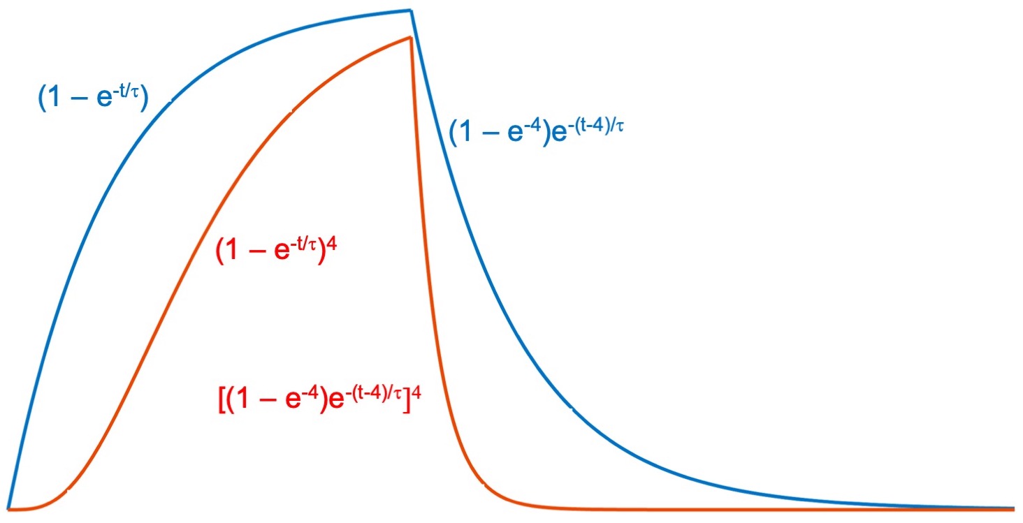
n. By raising
m to the third power and
n to the fourth, they ensure the conductances turn on slowly with a sigmoidal shape, but turn off abruptly, just as they found in paper 3. The
h-gate describes sodium inactivation, as reported in paper 4. The model not only reproduces their voltage clamp data, but also it predicts the action potential, all-or-none behavior, the refractory period, and even
anode break excitation.
 |
| The calculated (top) and measured (bottom) action potential. Adapted from Fig. 12 of Hodgkin & Huxley (1952). |
Wow! That’s an amazing set of papers.