Friday, October 17, 2014

A Theoretical Model of Magneto-Acoustic Imaging of Bioelectric Currents

Twenty years ago, I became interested in magneto-acoustic imaging, primarily influenced by the work of Bruce Towe that was called to my attention by my dissertation advisor and collaborator John Wikswo. (See, for example, Towe and Islam, “A Magneto-Acoustic Method for the Noninvasive Measurement of Bioelectric Currents,” IEEE Trans. Biomed. Eng., Volume 35, Pages 892–894, 1988). The result was a paper by Wikswo, Peter Basser, and myself (“A Theoretical Model of Magneto-Acoustic Imaging of Bioelectric Currents,” IEEE Trans. Biomed. Eng., Volume 41, Pages 723–728, 1994). This was my first foray into biomechanics, a subject that has become increasingly interesting to me, to the point where now it is the primary focus of my research (but that’s another story; for a preview look here).

A Treatise on the Mathematical Theory of Elasticity, by A. E. H. Love, superimposed on Intermediate Physics for Medicine and BIology.
A Treatise on the Mathematical
Theory of Elasticity,
by A. E. H. Love.
I started learning about biomechanics mainly through my friend Peter Basser. We both worked at the National Institutes of Health in the early 1990s. Peter used continuum models in his research a lot, and owned a number of books on the subject. He also loved to travel, and would often use his leftover use-or-lose vacation days at the end of the year to take trips to exotic places like Kathmandu. When he was out of town on these adventures, he left me access to his personal library, and I spent many hours in his office reading classic references like Schlichting’s Boundary Layer Theory and Love’s A Treatise on the Mathematical Theory of Elasticity. Peter and I also would read each other’s papers, and I learned much continuum mechanics from his work. (NIH had a rule that someone had to sign a form saying they read and approved a paper before it could be submitted for publication, so I would give my papers to Peter to read and he would give his to me.) In this way, I became familiar enough with biomechanics to analyze magneto-acoustic imaging. Interestingly, we published our paper in the same year Basser began publishing his research on MRI diffusion tensor imaging, for which he is now famous (see here).

As with much of my research, our paper on magneto-acoustic imaging addressed a simple “toy model”: an electric dipole in the center of an elastic, conducting sphere exposed to a uniform magnetic field. We were able to calculate the tissue displacement and pressure analytically for the cases of a magnetic field parallel and perpendicular to the dipole. One of my favorite results in the paper was that we found a close relationship between magneto-acoustic imaging and biomagnetism.
“Magneto-acoustic pressure recordings and biomagnetic measurements image action currents in an equivalent way: they both have curl J [the curl of the current density] as their source.”
For about ten years, our paper had little impact. A few people cited it, including Amalric Montalibet and later Han Wen, who each developed a method to use ultrasound and the Lorentz force to generate electrical current in tissue. I’ve described this work before in a review article about the role of magnetic forces in medicine and biology, which I have mentioned before in this blog. Then, in 2005 Bin He began citing our work in a long list of papers about magnetoacoustic tomography with magnetic induction, which again I've written about previously. His work generated so much interest in our paper that in 2010 alone it was cited 19 times according to Google Scholar. Of course, it is gratifying to see your work have an impact.

But the story continues with a more recent study by Pol Grasland-Mongrain of INSERM in France. Building on Montalibet’s work, Grasland-Mongrain uses an ultrasonic pulse and the Lorentz force to induce a voltage that he can detect with electrodes. The resulting electrical data can then be analyzed to determine the distribution of electrical conductivity (see Ammari, Grasland-Mongrain, et al. for one way to do this mathematically). In many ways, their technique is in competition with Bin He’s MAT-MI as a method to image conductivity.

Grasland-Mongrain also publishes his own blog about medical imaging. (Warning: The website is in French, and I have to rely on Google Translate to read it. It is my experience that Google has a hard time translating technical writing). There he discusses his most recent paper about imaging shear waves using the Lorentz force. Interestingly, shear waves in tissue is one of the topics Russ Hobbie and I added to the 5th edition of Intermediate Physics for Medicine and Biology, due out next year. Grasland-Mongrain’s work has been highlighted in Physics World and Focus Physics, and a paper about it appeared this year in Physical Review Letters, the most prestigious of all physics journals (and one I’ve never published in, to my chagrin).

I am amazed by what can happen in twenty years.


As a postscript, let me add a plug for toy models. Russ and I use a lot of toy models in IPMB. Even though such simple models have their limitations, I believe they provide tremendous insight into physical phenomena. I recently reviewed a paper in which the authors had developed a very sophisticated and complex model of a phenomena, but examination of a toy model would have told them that the signal they calculated was far, far to small to be observable. Do the toy model first. Then, once you have the insight, make your model more complex.

Friday, October 10, 2014

John H Hubbell

In the references at the end of Chapter 15 (Interaction of Photons and Charged Particles with Matter) in the 4th edition of Intermediate Physics for Medicine and Biology, you will find a string of publications authored by John H. Hubbell (1925–2007), covering a 27-year period from 1969 until 1996. Data from his publications are plotted in Fig. 15.2 (Total cross section for the interactions of photons with carbon vs. photon energy), Fig. 15.3 (Cross sections for the photoelectric effect and incoherent and coherent scattering from lead), Fig. 15.8 (The coherent and incoherent differential cross sections as a function of angle for 100-keV photons scattering from carbon, calcium, and lead), Fig. 15.14 (Fluorescence yields from K-, L-, and M-shell vacancies as a function of atomic number Z), and Fig. 15.16 (Coherent and incoherent attenuation coefficients and the mass energy absorption coefficient for water).

Hubbell’s 1982 paper “Photon Mass Attenuation and Energy-Absorption Coefficients from 1 keV to 20 MeV” (International Journal of Applied Radiation and Isotopes, Volume 33, Pages 1269–1290) has been cited 976 times according to the Web of Science. It has been cited so many times that it was selected as a citation classic, and Hubbell was invited to write a one-page reminiscence about the paper. It began modestly
Some papers become highly cited due to the creativity, genius, and vision of the authors, presenting seminal work stimulating and opening up new and multiplicative lines of research. Another, more pedestrian class of papers is “house-by-the-side-of-the-road” works, highly cited simply because these papers provide tools required by a substantial number of researchers in a single discipline or perhaps in several diverse disciplines, as is here the case.
At the time of his death, the International Radiation Physics Society Bulletin published the following obituary
The International Radiation Physics Society (IRPS) lost one of its major founding members, and the field of radiation physics one of its advocates and contributors of greatest impact, with the death this spring of John Hubbell.

John was born in Michigan in 1925, served in Europe in World War II [he received a bronze star], and graduated from the University of Michigan with a BSE (physics) in 1949 and MS (physics) in 1950. He then joined the National Bureau of Standards (NBS), later NIST, where he worked during his entire career. He married Jean Norford in 1955, and they had three children. He became best known and cited for National Standards Reference Data Series Report 29 (l969), “Photon Cross Sections, Attenuation Coefficients, and Energy Absorption Coefficients from 10 keV to 100 GeV.” He was one of the two leading founding members of the International Radiation Physics Society in 1985, and he served as its President 1994–97. While he retired from NIST in 1988, he remained active there and in the affairs of IRPS, until the stroke that led to his death this year.
Learn more about John Hubbell here and here.

Friday, October 3, 2014

Update on the 5th edition of IPMB

A few weeks ago, Russ Hobbie and I submitted the 5th edition of Intermediate Physics for Medicine and Biology to our publisher. We are not done yet; page proofs should arrive in a few months. The publisher is predicting a March publication date. I suppose whether we meet that target will depend on how fast Russ and I can edit the page proofs, but I am nearly certain that the 5th edition will be available for fall 2015 classes (for summer 2015, I am hopeful but not so sure). In the meantime, use the 4th edition of IPMB.

What is in store for the 5th edition? No new chapters; the table of contents will look similar to the 4th edition. But there are hundreds—no, thousands—of small changes, additions, improvements, and upgrades. We’ve included many new up-to-date references, and lots of new homework problems. Regular readers of this blog may see some familiar additions, which were introduced here first. We tried to cut as well as add material to keep the book the same length. We won’t know for sure until we see the page proofs, but we think we did a good job keeping the size about constant.

We found several errors in the 4th edition when preparing the 5th. This week I updated the errata for the 4th edition, to include these mistakes. You can find the errata at the book website, https://sites.google.com/view/hobbieroth. I won’t list here the many small typos we uncovered, and all the misspellings of names are just too embarrassing to mention in this blog. You can see the errata for those. But let me provide some important corrections that readers will want to know about, especially if using the book for a class this fall or next winter (here in Michigan we call the January–April semester "winter"; those in warmer climates often call it spring).
  • Page 78: In Problem 61, we dropped a key minus sign: “90 mV” should be “−90 mV”. This was correct in the 3rd edition (Hobbie), but somehow the error crept into the 4th (Hobbie and Roth). I can’t figure out what was different between the 3rd and 4th editions that could cause such mistakes to occur.
  • Page 137: The 4th edition claimed that at a synapse the neurotransmitter crosses the synaptic cleft and “enters the next cell.” Generally a neurotransmitter doesn’t “enter” the downstream cell, but is sensed by a receptor in the membrane that triggers some response.
  • Page 338: I have already told you about the mistake in the Bessel function identity in Problem 10 of Chapter 12. For me, this was THE MOST ANNOYING of all the errors we have found. 
  • Page 355: In Problem 12 about sound and hearing, I used an unrealistic value for the threshold of pain, 10−4 W m−2. Table 13.1 had it about right, 1 W m−2. The value varies between people, and sometimes I see it quoted as high as 10 W m−2. I suggest we use 1 W m−2 in the homework problem. Warning: the solution manual (available to instructors who contact Russ or me) is based on the problem as written in the 4th edition, not on what it would be with the corrected value.
  • Page 355: Same page, another screw up. Problem 16 is supposed to show how during ultrasound imaging a coupling medium between the transducer and the tissue can improve transmission. Unfortunately, in the problem I used a value for the acoustic impedance that is about a factor of a thousand lower than is typical for tissue. I should have used Ztissue = 1.5 × 10⁶ Pa s m−1. This should have been obvious from the very low transmission coefficient that results from the impedance mismatch caused by my error. Somehow, the mistake didn’t sink in until recently. Again, the solution manual is based on the problem as written in the 4th edition.
  • Page 433: Problem 30 in Chapter 15 is messed up. It contains two problems, one about the Thomson scattering cross section, and another (parts a and b) about the fraction of energy due to the photoelectric effect. Really, the second problem should be Problem 31. But making that change would require renumbering all subsequent problems, which would be a nuisance. I suggest calling the second part of Problem 30 as Problem “30 ½.” 
  • Page 523: When discussing a model for the T1 relaxation time in magnetic resonance imaging, we write “At long correlation times T1 is proportional to the Larmor frequency, as can be seen from Eq. 18.34.” Well, a simple inspection of Eq. 18.34 reveals that T1 is proportional to the SQUARE of the Larmor frequency in that limit. This is also obvious from Fig. 18.12, where a change in Larmor frequency of about a factor of three results in a change in T1 of nearly a factor of ten. 
  • Page 535: In Chapter 18 we discuss how the blood flow speed v, the repetition time TR, and the slice thickness Δz give rise to flow effects in MRI. Following Eq. 18.56, we take the limit when v is much greater than "TR/Δz". I always stress to my students that units are their friends. They can spot errors by analyzing if their equation is dimensionally correct. CHECK IF THE UNITS WORK! Clearly, I didn’t take my own advice in this case.
For all these errors, I humbly apologize. Russ and I redoubled our effort to remove mistakes from the 5th edition, and we will redouble again when the page proofs arrive. In the meantime, if you find still more errors in the 4th edition, please let us know. If the mistake is in the 4th edition, it could well carry over to the 5th edition if we don’t root it out immediately.

Friday, September 26, 2014

The First Steps in Seeing

The First Steps in Seeing,  by Robert Rodieck, superimposed on Intermediate Physics for Medicine and Biology.
The First Steps in Seeing,
by Robert Rodieck.
Russ Hobbie and I discuss the eye and vision in Chapter 14 of the 4th edition of Intermediate Physics for Medicine and Biology. But we just barely begin to describe the complexities of how we perceive light. If you want to learn more, read The First Steps in Seeing, by Robert Rodieck. This excellent book explains how the eye works. The preface states
This book is about the eyes—how they capture an image and convert it to neural messages that ultimately result in visual experience. An appreciation of how the eyes work is rooted in diverse areas of science—optics, photochemistry, biochemistry, cellular biology, neurobiology, molecular biology, psychophysics, psychology, and evolutionary biology. This gives the study of vision a rich mixture of breadth and depth.

The findings related to vision from any one of these fields are not difficult to understand in themselves, but in order to be clear and precise, each discipline has developed its own set of words and conceptual relations—in effect is own language—and for those wanting a broad introduction to vision, these separate languages can present more of an impediment to understanding than an aid. Yet what lies beneath the words usually has a beautiful simplicity.

My aim in this book is to describe how we see in a manner understandable to all. I’ve attempted to restrict the number of technical terms, to associate the terms that are used with a picture or icon that visually express what they mean, and to develop conceptual relations according to arrangements of these icons, or by other graphical means. Experimental findings have been recast in the natural world whenever possible, and broad themes attempt to bring together different lines of thought that are usually treated separately.

The main chapters provide a thin thread that can be read without reference to other books. They are followed by some additional topics that explore certain areas in greater depth, and by notes that link the chapters and topics to the broader literature.

My intent is to provide you with a framework for understanding what is known about the first steps in seeing by building upon what you already know.
Rodieck explains things in a quantitative, almost “physicsy” way. For instance, he imagines a person staring at the star Polaris, and estimates the number of photons (5500) arriving at the eye each tenth of a second (approximately the time required for visual perception), then determines their distribution on the retina, finds how many are at each wavelength, and how many per cone cell.

Color vision is analyzed, as are the mechanisms of how rhodopsin responds to a photon, how the photoreceptor produces a polarization of the neurons, how the retina responds with such a large dynamic range (“the range of vision extends from a catch rate of about one photon per photoreceptor per hour to a million per second”), and how eye movements hold an image steady on the retina. There’s even a discussion of photometry, with a table similar to the one I presented last week in this blog. I learned that the unit of retinal illuminance is the troland (td), defined as the luminance (candelas per square meter) times the pupil area (square millimeters).

Like IPMB, Rodieck ends his book with several appendices, including a first one on angles. His appendix on blackbody radiation includes in a figure showing the Planck function versus frequency plotted on log-log paper (I’ve always seen it plotted on linear axes, but the log-log plot helps clairfy the behavior at very large and small frequencies). The photon emission from the surface of a blackbody as a function of temperature is 1.52 × 10¹⁵ T3 photons per second per square meter (Rodieck does everything in terms of the number of photons). The factor of temperature cubed is not a typo; Stefan's law contains a T3 rather than T4 when written in terms of photon number. A lovely appendix analyzes the Poisson distribution, and another compares frequency and wavelength distributions.

The best feature of The First Steps in Seeing are the illustrations. This is a beautiful book. I suspect Rodieck read Edward Tufte’s the Visual Display of Quantitative Information, because his figures and plots elegantly make his points with little superfluous clutter. I highly recommend this book.

Friday, September 19, 2014

Lumens, Candelas, Lux, and Nits

In Chapter 14 (Atoms and Light) of the 4th edition of Intermediate Physics for Medicine and Biology, Russ Hobbie and I discuss photometry, the measurement of electromagnetic radiation and its ability to produce a human visual sensation. I find photometry interesting mainly because of all the unusual units.

Let’s start by assuming you have a source of light emitting a certain amount of energy per second, or in other words with a certain power in watts. This is called the radiant power or radiant flux, and is a fundamental concept in radiometry. But how do we perceive such a source of light? That is a question in photometry. Our perception will depend on the wavelength of light. If the light is all in the infrared or ultraviolet, we won’t see anything. If in the visible spectrum, our perception depends on the wavelength. In fact, the situation is even more complicated than this, because our perception depends on if we are using the cones in the retina of our eye to see bright light in color (photopic vision), or we are using rods to see dim light in black and white (scotopic vision). Moreover, our ability to see varies among individuals. The usual convention is to assume we are using photopic vision, and to say that a source radiating a power of one watt of light at a wavelength of 555 nm (green light, the wavelength that the eye is most sensitive to) has a luminous flux of 683 lumens.

The light source may emit different amounts of light in different directions. In radiometry, the radiant intensity is the power emitted per solid angle, in units of watt per steradian. We can define an analogous photometric unit for the luminous intensity to be the luman per steradian, or the candela. The candela is one of seven “SI base units” (the others are the kilogram, meter, second, ampere, mole, and kelvin). Russ and I mention the candela in Table 14.6, which is a large table that compares radiometric, photometric and actinometric quantities. We also define it in the text, using the old-fashioned name “candle” rather than candela.

Often you want to know the intensity of light per unit area, or irradiance. In radiometry, irradiance is measured in watts per square meter. In photometry, the illuminance is measured in lumens per square meter, also called the lux.

Finally, the radiance of a surface is the radiant power per solid angle per unit surface area (W sr−1 m−2). The analogous photometric quantity is the luminance, which is measured in units of lumen sr−1 m−2, or candela m−2, or lux sr−1, or nit. The brightness of a computer display is measured in nits.

In summary, below is an abbreviated version of Table 14.6 in IPMB
Radiometry Photometry
Radiant power (W) Luminous flux (lumen)
Radiant Intensity (W sr−1) Luminous intensity (candela)
Irradiance (W m−2) Illuminance (lux)
Radiance (W sr−1 m−2) Luminance (nit)
Where did the relationship between 1 W and 683 lumens come from? Before electric lights, a candle was a major source of light. A typical candle emits about 1 candela of light. The relationship between the watt and the lumen is somewhat analogous to the relationship between absolute temperature and thermal energy, and the relationship between a mole and the number of molecules. This would put the conversion factor of 683 lumens per watt in the same class as Boltzmann's constant (1.38 × 10⁻²³ J per K) and Avogadro's number (6.02 × 10²³ molecules per mole).

Friday, September 12, 2014

More about the Stopping Power and the Bragg Peak

The Bragg peak is a key concept when studying the interaction of protons with tissue. In Chapter 16 of the 4th edition of Intermediate Physics for Medicine and Biology, Russ Hobbie and I write
Protons are also used to treat tumors. Their advantage is the increase of stopping power at low energies. It is possible to make them come to rest in the tissue to be destroyed, with an enhanced dose relative to intervening tissue and almost no dose distally (“downstream”) as shown by the Bragg peak in Fig. 16.51 [see a similar figure here]. Placing an absorber in the proton beam before it strikes the patient moves the Bragg peak closer to the surface. Various techniques, such as rotating a variable-thickness absorber in the beam, are used to shape the field by spreading out the Bragg peak (Fig. 16.52) [see a similar figure here].
Figure 16.52 is very interesting, because it shows a nearly uniform dose throughout a region of tissue produced by a collection of Bragg peaks, each reaching a maximum at a different depth because the protons have different initial energies. The obvious question is: how many protons should one use for each energy to produce a uniform dose in some region of tissue? I have discussed the Bragg peak before in this blog, when I presented a new homework problem to derive an analytical expression for the stopping power as a function of depth. An extension of this problem can be used to answer this question. Russ and I considered including this extended problem in the 5th edition of IPMB (which is nearing completion), but it didn’t make the cut. Discarded scraps from the cutting room floor make good blog material, so I present you, dear reader, with a new homework problem.
Problem 31 3/4 A proton of kinetic energy T is incident on the tissue surface (x = 0). Assume its stopping power s(x) at depth x is given by
An equation showing the stopping power as a function of depth. This equation illustrates the Bragg peak.
where C is a constant characteristic of the tissue.
(a) Plot s(x) versus x. Where does the Bragg peak occur?
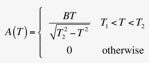
(b) Now, suppose you have a distribution of N protons. Let the number with incident energy between T and T+dT be A(T)dT, where
An equation giving the distribution of proton energies in this example of spreading out the Bragg peak.
Determine the constant B by requiring
An equation showing how to normalize the distribution of proton energies.
Plot A(T) vs T.
(c) If x is greater than T22/2C what is the total stopping power? Hint: think before you calculate; how many particles can reach a depth greater than T22/2C?

(d) If x is between T12/2C and T22/2C, only particles with energy from (2Cx)1/2 to T2 contribute to the stopping power at x, so
An integral giving the stopping power as a function of position.
Evaluate this integral. Hint: let u = T2 - (2Cx + T22)/2.
(e) If x is less than T12/2C, all the particles contribute to the stopping power at x, so
An integral giving the stopping power as a function of position.
Evaluate this integral.

(f) Plot S(x) versus x. Compare your plot with that found in part a, and with Fig. 16.52.
One reason this problem didn’t make the cut is that it is rather difficult. Let me know if you need the solution. The bottom line: this homework problem does a pretty good job of explaining the results in Fig. 16.52, and provides insight into how to apply proton therapy to an large tumor.

Friday, September 5, 2014

Raymond Damadian and MRI

The 2003 Nobel Prize in Physiology or Medicine was awarded to Paul Lauterbur and Sir Peter Mansfield “for their discoveries concerning magnetic resonance imaging.” In Chapter 18 of the 4th Edition of Intermediate Physics for Medicine and Biology, Russ Hobbie and I discuss MRI and the work behind this award. Choosing Nobel Prize winners can be controversial, and in this case some suggest that Raymond Damadian should have shared in the prize. Damadian himself famously took out an ad in the New York Times claiming his share of the credit. Priority disputes are not pretty events, but one can gain some insight into the history of magnetic resonance imaging by studying this one. The online news source Why Files tells the story in detail. The controversy continues even today (see, for instance, the website of Damadian's company FONAR). Unfortunately, Damadian’s religious beliefs have gotten mixed up in the debate.

I think the issue comes down to a technical matter about MRI. If you believe the variation of T1 and T2 time constants among different tissues is the central insight in developing MRI, then Damadian has a valid claim. If you believe the use of magnetic field gradients for encoding spatial location is the key insight in MRI, his claim is weaker than Lauterbur and Mansfield's. Personally, I think the key idea of magnetic resonance imaging is using magnetic field gradients. IPMB states
“Creation of the images requires the application of gradients in the static magnetic field Bz which cause the Larmor frequency to vary with position.”
My understanding of MRI history is that this idea originated with Lauterbur and Mansfield (and was also earlier discovered by Hermann Carr).

To learn more, I suggest you read Naked to the Bone, which I discussed previously in this blog. This book discusses both the Damadian controversy, and a similar controversy centered around William Oldendorf and the development of computed tomography (which is mentioned in IPMB).

Friday, August 29, 2014

Student’s T Test

Primer of Biostatistics, by Stanton Glantz, superimposed on Intermediate Physics for Medicine and Biology.
Primer of Biostatistics,
by Stanton Glantz.
Probability and statistics is an important topic in medicine. Russ Hobbie and I discuss probability in the 4th edition of Intermediate Physics for Medicine and Biology, but we don’t delve into statistics. Yet, basic statistics is crucial for analyzing biomedical data, such as the results of a clinical trial.

Suppose IPMB did contain statistics. What would that look like? I suspect Russ and I would summarize this topic in an appendix. The logical place seems to be right after Appendix G (The Mean and Standard Deviation). We would probably not want to go into great detail, so we would only consider the simplest case: a “student’s t-test” of two data sets. It would be something like this (but probably less wordy).
Appendix G ½  Student’s T Test

Suppose you divide a dozen patients into two groups. Six patients get a drug meant to lower their blood pressure, and six others receive a placebo. After receiving the drug for a month, their blood pressure is measured. The data is given in Table G ½.1.

Table G ½.1. Systolic Blood Pressure (in mmHg)
Drug Placebo
115   99
  90 106
  99 100
108 119
107   96
  96 104

Is the drug effective in lowering blood pressure? Statisticians typically phrase the question differently: they adopt the null hypothesis that the drug has no effect, and ask if the data justifies the rejection of this hypothesis.

The first step is to calculate the mean, using the methods described in Appendix G. The mean for those receiving the drug is 102.5 mmHg, and the mean for those receiving the placebo is 104.0 mmHg. So, the mean systolic blood pressure was lower with the drug. The crucial question is: could this difference arise merely from chance, or does it represent a real difference? In other words, is it likely that this difference is a coincidence caused by taking too small of a sample?

To answer this question, we need to next calculate the standard deviation σ of each data set. We calculate this using Eq. G.4, except that because we do not know the mean of the data but only estimate it from our sample, we should use the factor N/(N-1) for the best estimate of the variance, where N = 6 in this example. The standard deviation is then σ = √( Σ (x -xmean)2/(N-1) ). The calculated standard deviation for the patients who took the drug is 9.1, whereas for the patients who took the placebo it is 8.2. 

The standard deviation describes the spread of the data within the sample, but what we really care about is how accurately we know the mean of the data. The standard deviation of the mean is calculated by dividing the standard deviation by the square root of N. This gives 3.7 for patients taking the drug, and 3.3 for patients taking the placebo.

We are primarily interested in the difference of the means, which is 104.0 – 102.5 = 1.5 mmHg. The standard deviation of the difference in the means can be found by squaring each standard deviation of the mean, adding them, and taking the square root (standard deviations add like in the Pythagorean theorem). You get
√(3.72 + 3.32) = 5.0 mmHg.

Compare the difference of the means to the standard deviation of the difference of the means by taking their ratio. Following tradition we will call this ratio T, so T = 1.5/5.0 = 0.3. If the drug has a real effect, we would expect the difference of the mean to be much larger than the standard deviation of the difference of the mean, so the absolute value of T should be much greater than 1. On the other hand, if the difference of means is much smaller than the standard deviation of the difference of the means, the result could arise easily from chance and |T| should be much less than 1. Our value is 0.3, which is less than 1, suggesting that we cannot reject the null hypothesis, and that we have not shown that the drug has any effect. 

But can we say more? Can we transform our value of T into a probability that the null hypothesis is true? We can. If the drug truly had no effect, then we could repeat the experiment many times and get a distribution of T values. We would expect the values of T to be centered about T = 0 (remember, T can be positive or negative), with small values much more common than large. We could interpret this as a probability distribution: a bell shaped curve peaked at zero and falling as T becomes large. In fact, although we will not go into the details here, we can determine the probability that |T| is greater than some critical value. By tradition, one usually requires the probability p to be larger than one twentieth (p greater than 0.05) if we want to reject the null hypothesis and claim that the drug does indeed have a real effect. The critical value of T depends on N, and values are tabulated in many places (for example, see here). In our case, the tables suggest that T would have to be greater than 2.23 in order to reject the null hypothesis and say that the drug has a true (or, in the technical language, a “significant”) effect.

If taking p greater than 0.05 seems like an arbitrary cutoff for significance, then you are right. Nothing magical happens when p reaches 0.05. All it means is that the probability that the difference of the means could have arisen by chance is less than 5%. It is always possible that you were really, really unlucky and that your results arose by chance but |T| just happened to be very large. You have to draw a line somewhere, and the accepted tradition is that p greater than 0.05 means that the probability of the results being caused by random chance is small enough to ignore. 

Problem 1 Analyze the following data and determine if X and Y are significantly different. 
  X  Y
  94 122
  93 118
104 119
105 123
115 102
  96 115
Use the table of critical values for the T distribution at
http://en.wikipedia.org/wiki/Student%27s_t-distribution.
I should mention a few more things.

1. Technically, we consider above a two-tailed t-test, so we’re testing if we can reject the null hypothesis that the two means are the same, implying that either the drug had a significant effect of lowering blood pressure or the drug had a significant effect of raising blood pressure. If we wanted to test only if the drug lowered blood pressure, we should use a one-tailed test.

2. We analyzed what is known as an unpaired test. The patients who got the drug are different than the patients who did not. Suppose we gave the drug to the patients in January, let them go without the drug for a while, then gave the same patients the placebo in July (or vice versa). In that case, we have paired data. It may be that patients vary a lot among themselves, but that the drug reduced everyone’s blood pressure by the same fixed percentage, say 12%. There are special ways to generalize the t-test for paired data.

3. It’s easy to generalize these results to the case when the two samples have different numbers N.

4. Please remember, if you found 20 papers in the literature that all observed significant effects with p less than but on the order of 0.05, then on average one of those papers is going to be reporting a spurious result: the effect is reported as significant when in fact it is a statistical artifact. Given that there are thousands (millions?) of papers out there reporting the results of t-tests, there are probably hundreds (hundreds of thousands?) of such spurious results in the literature. The key is to remember what p means, and to not over-interpret or under-interpret your results.

5. Why is this called the “student’s t-test”? The inventor of the test, William Gosset, was a chemist working for Guinness, and he devised the t-test to assess the quality of stout. Guinness would not let its chemists publish, so Gosset published under the pseudonym “student.”

6. The t-test is only one of many statistical methods. As is typical of IPMB, we have just scratched the surface of an exciting and extensive topic. 

7. There are many good books on statistics. One that might be useful for readers of IPMB (focused on biological and medical examples, written in engaging and nontechnical prose) is Primer of Biostatistics, 7th edition, by Stanton Glantz.

Friday, August 22, 2014

Point/Counterpoint: Low-Dose Radiation is Beneficial, Not Harmful

I have discussed the pedagogical virtues of point/counterpoint articles published by Medical Physics before in this blog (see, for instance, here and here). They are a wonderful resource to augment any medical physics class, and serve as an excellent supplement to the 4th edition of Intermediate Physics for Medicine and Biology. Medical Physics posts all its point/counterpoint articles freely available online (open access). Each article presents a somewhat controversial proposition in the title, and two leading medical physicists then debate the issue, one pro and one con. Each makes an opening statement, and each has a chance to respond to their opponents opening statement in a rebuttal.

One example that is closely related to a topic in IPMB is addressed in the July 2014 point/counterpoint article, which debates the proposition that “low-dose radiation is beneficial, not harmful.” Mohan Doss argues for the proposition, and Mark Little argues against it. The issue is central to the “linear no threshold” model of radiation risk that Russ Hobbie and I discuss in Sec. 16.13 (The Risk of Radiation) of IPMB. Mohan Doss leads off with this claim:
When free radical production is increased, e.g., from low-dose radiation (LDR) exposure (or increased physical/mental activity), our body responds with increased defenses consisting of increased antioxidants, DNA repair enzymes, immune system response, etc. referred to as adaptive protection. With enhanced protection, there would be reduced cumulative damage in the long term and reduced diseases. The disease-preventive effects of increased physical/mental activities are well known.
Little responds:
Dr. Doss discusses the well-known involvement of the immune system in cancer, and more generally the role of adaptive response. The critical issue is whether the up-regulation of the immune system or other forms of adaptive response that may result from a radiation dose offsets the undoubted carcinogenic damage that is caused. The available evidence, summarized in my Opening Statement, is that it does not.
Both cite the literature extensively. I find it fascinating that such a basic hypothesis hasn’t, to this day, been resolved. We don’t even know the sign of the effect: is low dose radiation positive or negative for our health. Although I can’t tell you who is right, Doss or Little, I can tell you who wins: the reader. And especially the student, who gets a front-row seat at a cutting-edge scientific debate between two world-class experts.

By the way, point/counterpoint articles aren’t the only articles available free-of-charge at the Medical Physics website. You can get 50th Anniversary Papers [for its 50th anniversary, Medical Physics published several retrospective papers], Vision 20/20 papers [summaries of state-of-the-art developments in medical physics], award papers, special focus papers, and more. And it’s all free.

I love free stuff.

Friday, August 15, 2014

Physics of Phoxhounds

I don’t have any grandchildren yet, but I am fortunate to have a wonderful “granddog.” This weekend, my wife and I are taking care of Auggie, the lovable foxhound that my daughter Kathy rescued from an animal shelter in Lansing, Michigan. Auggie gets along great with our Cocker-Westie mix, “Aunt Suki,” my dog-walking partner who I’ve mentioned often in this blog (here, here, here, and here).

Do dogs and physics mix? Absolutely! If you don’t believe me, then check out the website dogphysics.com. I plan to read “How To Teach Physics To Your Dog” with Auggie and Suki. According to this tee shirt foxhounds are particularly good at physics. Once we finish “How To Teach Physics To Your Dog,” we may move on to “Physics for Dogs: A Crash Course in Catching Cats, Frisbees, and Cars.” Apparently there is even a band that sings about dog physics, but I don’t know what that is all about.

Auggie is a big fan of the 4th edition of Intermediate Physics for Medicine and Biology. His favorite part is Section 7.10 (Electrical Stimulation) because there Russ Hobbie and I discuss the “dog-bone” shaped virtual cathode that arises when you stimulate cardiac tissue using a point electrode. He thinks “Auger electrons,” discussed in Sec. 17.11, are named after him. Auggie’s favorite scientist is Godfrey Hounsfield (Auggie adds a “d” to his name: “Houndsfield”), who earned a Nobel Prize for developing the first clinical computed tomography machine. And his favorite homework problem is Problem 34 in Chapter 2, about the Lotka-Volterra equations governing the population dynamics of rabbits and foxes.

How did Auggie get his name? I’m not sure, because he had the name Auggie when Kathy adopted him. I suspect it comes from an old Hanna-Barbera cartoon about Augie Doggie and Doggie Daddy. When Auggie visits, I get to play doggie [grand]daddy, and say “Augie, my son, my son” in my best Jimmy Durante voice. I’m particularly fond of the Augie doggie theme song. What is Auggie’s favorite movie? Why, The Fox and the Hound, of course.

A photograph of Brad Roth holding his dog Suki Roth in Michigan's fall color.
Me holding Suki.
Our dog Suki has some big news this week. My friend and Oakland University colleague Barb Oakley has a new book out: A Mind for Numbers: How to Excel at Math and Science (Even if You Flunked Algebra). I contributed a small sidebar to the book offering some tips for learning physics, and it includes a picture of me with Suki! Thanks to my friend Yang Xia for taking the picture. Barb is a fascinating character and author of an eclectic collection of books. I suggest Hair of the Dog: Tails from Aboard a Russian Trawler. Her amazon.com author page first gave me the idea of publishing a blog to go along with IPMB. To those of you who are interested in physics applied to medicine and biology but struggle with all the equations in IPMB, I suggest Barb's book or her MOOC Learning How to Learn.

All Creatures Great and Small, by James Herriot, superimposed on Intermediate Physics for Medicine and Biology.
All Creatures Great and Small,
by James Herriot.
James Herriot—the author of a series of wonderful books including All Creatures Great and Small, which will warm the heart of any dog-lover—loved beagles, which look similar to foxhounds, but are smaller. If you’re looking for an uplifting and enjoyable book to read on a late-summer vacation (and you have already finished IPMB), try Herriot’s books. But skip the chapters about cats (yuck).

Auggie may not be the brightest puppie in the pack, and he is too timid to be an effective watch dog, but he has a sweet and loving disposition. I think of him as a gentle soul (even if he did chew up his grandma’s shoe). Below is a picture of Auggie and his Aunt Suki, getting ready for their favorite activity: napping.

Suki Roth with the lovable foxhound Auggie, napping.
Suki and Auggie.