The activity A(t) is the number of radioactive transitions
(or transformations or disintegrations) per second. The SI
unit of activity is the becquerel (Bq):
1 Bq = 1 transition s−1.
The earlier unit of activity, which is still used occasionally,
is the curie (Ci):
1 Ci=3.7 × 10¹⁰ Bq,
1 μCi = 3.7 ×10⁴ Bq.
Several excellent articles were published about Marie Curie and her husband/collaborator Pierre Curie for the centennial of her 1898 discovery of radium. Saenger and Adamek’s article in the journal Medical Physics states
Marie Curie’s activities and research left her imprint on
nuclear medicine, which continues to this day. Much of her
impact is related to the role of women in science, biology,
and medicine. She successfully overcame struggles for recognition
in the first decades of this century. One of her major
achievements was the development of field-radiography for
wounded soldiers in World War I. Her continued endeavors
to provide radium therapy for cancer was a giant step for
humanity. She worked unceasingly in the laboratory to separate
and identify radioactive elements of the periodic table.
The standardization of these elements resulted in the 1931
report of the International Radium-Standards Commission
and the posthumous two-volume Radio-aktivite´.
This review celebrates the events of 100 years ago to the month of publication of this December 1998 issue of the British Journal of Radiology, when radium was discovered by the Curies. This followed the earlier discovery in November 1895 of X-rays by Röntgen, which has already been reviewed in the British Journal of Radiology [1] and the discovery in March 1896, by Becquerel, of the phenomenon of radioactivity, which introduces this review. This is particularly relevant as Marie Curie was in 1897 a research student in Becquerel’s laboratory. Marie Curie’s life in Poland prior to her 1891 departure for Paris is included in this review as are other aspects of her life and work such as her work in World War I with radiological ambulances (known as “Little Curies”) on the battlefields of France and Belgium, early experiments with radium and the founding of the Institut du Radium in Paris and of the Radium Institute in Warsaw. Wherever possible I have included appropriate quotations in Marie Curie’s own words [2–4] and each section is related in some way to the life and work of Maria or Pierre. This review is completed with details of the re-interment of the bodies of Pierre and Marie on 20 April 1995 in The Panthéon, Paris.
Excellent overviews of Curie’s life and work are provided by the AIP Center for the History of Physics and the Official Website of the Nobel Prize. You can read about the discovery of radium in Maria Curie’s own words here. And for all you dear readers who prefer Saturday morning cartoons to learned articles, watch this; it doesn’t include any complex or controversial stuff like the Langevin affair, but it is enjoyable in its own simple way.
Recently, the visual artist/filmmaker/writer Quintan Ana Wikswo was granted access to Marie Curie’s laboratory in Paris for “creating performance films and photographs for ... LUMINOSITY: THE PASSIONS OF MARIE CURIE, a multimedia opera by composer Pamela Madsen.” Wikswo describes her ongoing work and previews some of her photographs in her blog Bumblemoth.
To see her books, her equipment, to stand at her desk, to see her beakers and centrifuges and shelves of chemicals…it’s a kind of searing existential therapy, and anyone visiting Paris should make the effort to spend a few moments at her lab. Why? It’s an antidote, at the very least. I work half-days at her lab, and then explore art museums of Paris in the off hours. The contrast is shocking and disturbing. Inspiring and sorrowful.
At Oakland University, I work in the College of “Arts and Sciences.” Wikswo has found her own niche at the intersection of these two rarely-overlapping endeavors. I look forward to seeing the completed project.
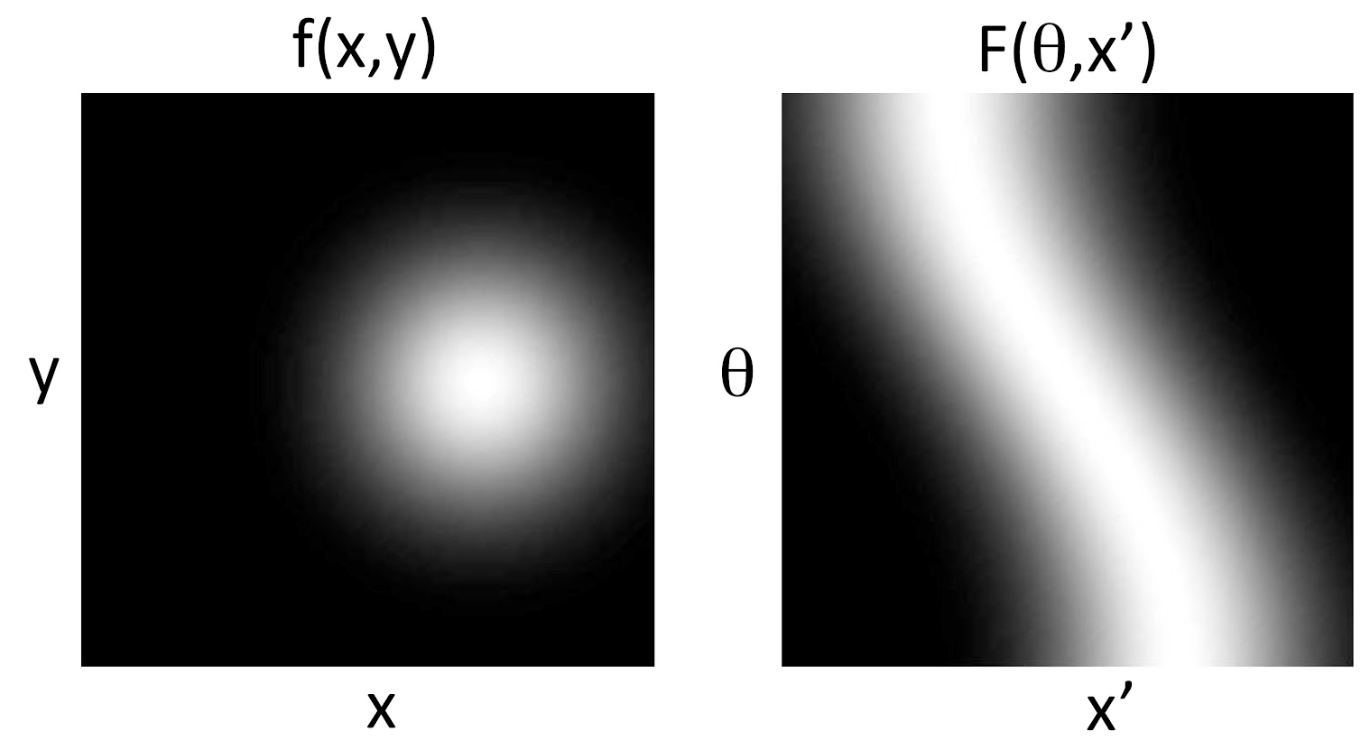
I love sinograms. They are rare and fascinating mixtures of science and art, and often are quite beautiful. One should be able to look at a sinogram and intuitively picture the two-dimensional image. Unfortunately, I rarely can do this, except for the most simple examples.
Russ Hobbie and I define the sinogram in the 4th edition of Intermediate Physics for Medicine and Biology. We explain how to calculate the projection, F(θ, x'), from the image, f(x,y). This transformation and its inverse—determining f(x,y) from F(θ,x')—is at the heart of many imaging algorithms, such as those used in computed tomography.
The process of calculating F(θ, x') from f(x, y) is sometimes
called the Radon transformation. When F(θ, x') is
plotted with x’ on the horizontal axis, θ on the vertical
axis, and F as the brightness or height on a third perpendicular
axis, the resulting picture is called a sinogram. For
example, the projection of f(x, y) = δ(x − x0)δ(y − y0)
is F(θ, x') = δ(x' − (x0 cos θ + y0 sin θ)). A plot of this
object and its sinogram is shown in Fig. 12.17.
Figure 12.17 does indeed contain a sinogram, but a very simple one: the sinogram of a point is just a sine wave. The reader is asked to produce a somewhat more complicated sinogram in homework Problem 29.
Problem 29An object consists of three δ functions at
(0, 2), (√3,−1), and (−√3,−1). Draw the sinogram of the object.
This sinogram consists of three braided sine waves. I like this example, because it’s simple enough that you the reader should be able to reason out the structure of the sinogram by imagining the projection in your head, but it is complicated enough that it’s not trivial.
When preparing the 4th edition of Intermediate Physics for Medicine and Biology, I derived a couple new homework problems (Chapter 12, Problems 23 and 24) for which the inverse transformation can be solved analytically. I think these are useful exercises that build intuition with the Fourier transform method of reconstructing an image (see Fig. 12.20, top path). It occurs to me now, however, that while these problems do provide insight and practice for the mathematically inclined reader, they also offer the opportunity to further illustrate the sinogram. So this week I made the figures below, showing the image f(x,y) on the left and the corresponding sinogram F(θ,x') on the right, for the functions in Problems 23 and 24.
Problem 23.
Problem 24.
Let us try to interpret these pictures qualitatively. The vertical axis in the sinogram (right panel) indicates the angle, specifying the direction of the projection (the direction that the x-rays come from, to use CT terminology). The bottom of the θ axis is an angle of zero indicating x-rays are incident on the image from the bottom, the middle of the θ axis is x-rays incident from the left, and the top of the θ axis is x-rays incident from the top (see Fig. 12.12). Some authors extend the θ axis so it ranges from 0 to 360°, but to me that seems unnecessary since having the x-rays come from one side or the opposite side does not matter; it provides no new information. It’s best if you, dear reader, pause now and stare at these sinograms until you understand how they relate to the image. If you really want to build your intuition, cover the left panel, and try to predict what the hidden image looks like from just the right panel. Or, solve homework Problems 30 and 31 in Chapter 12, and then plot both the image and its sinogram like I do above.
This website has some nice examples of sinograms. For instance, a sinogram of a line is just a point. Think about it and sketch some projections to convince yourself this is correct. Also this website shows a sinogram of a square located away from the center of the image (it looks like the sinogram above for Fig. 23, but with interesting bright curves tenuously weaving throughout the sinogram arising from the corners of the square). Finally, the website shows the sinogram of an image known as a Shepp-Logan head phantom. (Warning, the website displays its sinograms rotated by 90° compared to the way Russ and I plot them; it plots the angle along the horizontal axis.) The video shown below provides additional insight into the construction of the sinogram for the Shepp-Logan head phantom.
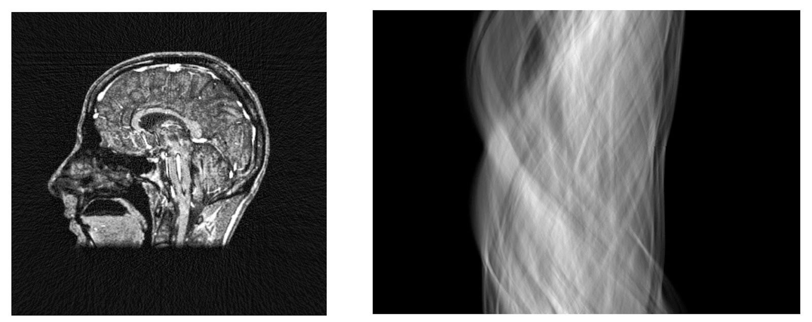
Here is one of my favorite images:
a detailed image of a brain, and its lovely
sinogram. If you can do the inverse transformation of this complicated
sinogram in your head, you’re a better medical physicist than I am.
An image of a brain, and its sinogram,
adapted from Wikipedia.
Problem 4 (a) Starting with Eq. 14.7, derive a formula for the hydrogen atom spectrum in the form
where n and m are integers. R is called the Rydberg constant. Find an expression for R in terms of fundamental constants.
(b) Verify that the wavelengths of the spectral lines a-d at the top of Fig. 14.3 are consistent with the energy transitions shown at the bottom of the figure.
Our Fig. 14.3 is in black and white. It is often useful to see the visible hydrogen spectrum (just four lines, b-e in Fig 14.3) in color, so you can appreciate better the position of the emission lines in the spectrum.
The hydrogen lines in the visible part of the spectrum are often referred to as the Balmer series, in honor of physicist Johann Balmer who discovered this part of the spectrum before Rydberg. Additional Balmer series lines exist in the near ultraviolet part of the spectrum (the thick band of lines just to the left of line e at the top of Fig. 14.3). All the Balmer series lines can be reproduced using the equation in Problem 4 with n = 2.
An entire series of spectral lines exists in the extreme ultraviolet, called the Lyman series, shown at the top of Fig. 14.3 as the line labeled a and the lines to its left. These lines are generated by the formula in Problem 4 using n = 1. The new homework problem below will help the student better understand the hydrogen spectrum.
Section 14.2
Problem 4 ½The Lyman series, part of the spectrum of hydrogen, is shown at the top of Fig. 14.3 as the line labeled a and the band of lines to the left of that line. Create a figure like Fig. 14.3, but which shows a detailed view of the Lyman series. Let the wavelength scale at the top of your figure range from 0 to 150 nm, as opposed to 0-2 μm in Fig. 14.3. Also include an energy level drawing like at the bottom of Fig. 14.3, in which you indicate which transitions correspond to which lines in the Lyman spectrum. Be sure to indicate the shortest possible wavelength in the Lyman spectrum, show what transition that wavelength corresponds to, and determine how this wavelength is related to the Rydberg constant.
Many spectral lines can be found in the infrared, known as the Paschen series (n = 3), the Brackett series (n = 4) and the Pfund series (n = 5). The Paschen series is shown as lines f, g, h, and i in Fig. 14.3, plus the several unlabeled lines to their left. The Paschen, Brackett, and Pfund series overlap, making the hydrogen infrared spectrum more complicated than its visible and ultraviolet spectra. In fact, the short-wavelength lines of the Brackett series would appear at the top of Fig. 14.3 if all spectral lines were shown.
Asimov's Biographical Encyclopedia of Science and Technology,
by Isaac Asimov.
RYDBERG, Johannes Robert (rid’bar-yeh)
Swedish physicist
Born: Halmstad, November 8, 1854.
Died: Lund, Malmohus, December 28, 1919.
Rydberg studied at the University of Lund and received his Ph.D. in mathematics in 1879, and then jointed the faculty, reaching professorial status in 1897.
He was primarily interested in spectroscopy and labored to make sense of the various spectral lines produced by the different elements when incandescent (as Balmer did for hydrogen in 1885). Rydberg worked out a relationship before he learned of Balmer’s equation, and when that was called to his attention, he was able to demonstrate that Balmer’s equation was a special case of the more general relationship he himself had worked out.
Even Rydberg’s equation was purely empirical. He did not manage to work out the reason why the equation existed. That had to await Bohr’s application of quantum notions to atomic structure. Rydberg did, however, suspect the existence or regularities in the list of elements that were simpler and more regular than the atomic weights and this notion was borne out magnificently by Moseley’s elucidation of atomic numbers.
Yesterday was the 158th anniversary of Rydberg’s birth.
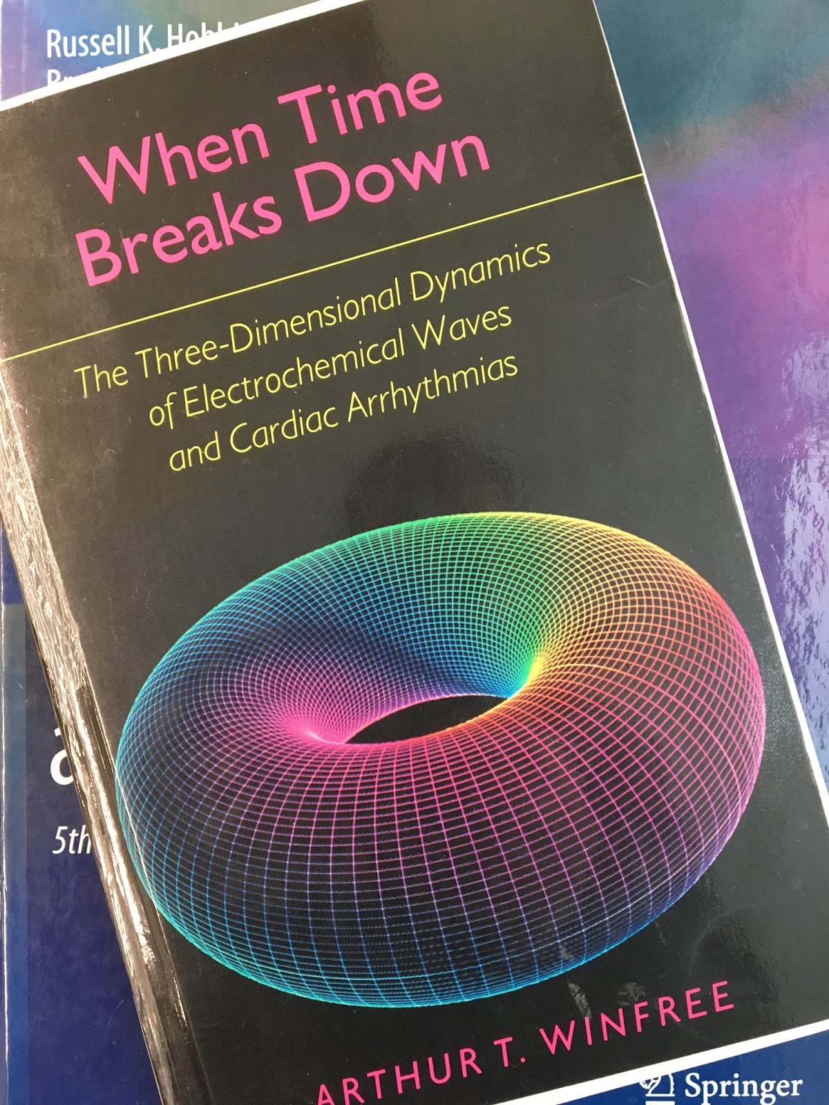
One place where Winfree’s work impacts our book is in Problems 39 and 40 in Chapter 10, discussing cellular automata. Winfree didn’t invent cellular automata, but his discussion of them in his wonderful book When Time Breaks Down is where I first learned about the topic.
Box 5.A: A Cellular Excitable Medium
Take a pencil and a sheet of tracing paper and play with Figure 5.2 [a
large hexagonal array of cells] according to the following game rules …
Each little hexagon in this honeycomb is supposed to represent a cell
that may be excited for the duration of one step (put a “0” in the cell)
or refractory (after the excited moment, replace the “0” with a “1”) or
quiescent (after that erase the “1”) until such time as any adjacent
cell becomes excited: then pencil in a “0” in the next step.
If you start with no “0’s,” you’ll never get any, and this simulation
will cost you little effort. If you start with a single “0” somewhere,
it will next turn to “1” while a ring of 6 neighbors become infected
with “0”. As the hexagonal ring of “0’s” propagates, it is followed by a
concentric ring of “1” refractoriness, right to the edge of the
honeycomb, where all vanish.
Now see what happens if you violate the rules just once by erasing a
segment of that ring wave when it is about halfway to the edges: you
will have created a pair of counter-rotating vortices (alias phase
singularities), each of which turns out to be a source of radially
propagating waves.
(Stop reading until you have played some.)
You may feel a bit foolish, since this is obviously supposed to mimic
action potential propagation, and the caricature is embarrassingly
crude. Which aspects of its behavior are realistic and which others are
merely telling us “honeycombs are not heart muscle”? The way to find out
is to undertake successively more refined caricatures until a point of
diminishing returns is reached. For most purposes, it is reached
surprisingly soon.
During a cathodal stimulus, the state of the cell directly under the
electrode and its four nearest neighbors in the direction perpendicular
to the fibers change to the excited state, and the two remaining nearest
neighbors in the direction parallel to the fibers change to the
quiescent state, regardless of their previous state.
Using this simple model, I was able to initiate “quatrefoil reentry” (Lin et al., 1999; read more here).
I also could reproduce most of the results of a simulation of the
“pinwheel experiment” (a point stimulus applied near the end of the
refractory period of a previous planar wave front) predicted by Lindblom et al. (2000). I concluded
This extremely simple cellular excitable medium—which is nothing more
than a toy model, stripped down to contain only the essential
features—can, with one simple modification for strong stimuli, predict
many interesting and important phenomena. Much of what we have learned
about virtual electrodes and deexcitation is predicted correctly by the
model (Efimov et al., 2000; Trayanova, 2001).
I am astounded that this simple model can reproduce the complex results
obtained by Lindblom et al. (2000). The model provides valuable insight
into the essential mechanisms of electrical stimulation without hiding
the important features behind distracting details.
When Art Winfree died in Tucson on November 5, 2002, at the age of 60,
the world lost one of its most creative scientists. I think he would
have liked that simple description: scientist. After all, he made it
nearly impossible to categorize him any more precisely than that. He
started out as an engineering physics major at Cornell (1965), but then
swerved into biology, receiving his PhD from Princeton in 1970. Later,
he held faculty positions in theoretical biology (Chicago, 1969–72), in
the biological sciences (Purdue, 1972–1986), and in ecology and
evolutionary biology (University of Arizona, from 1986 until his death).
So the eventual consensus was that he was a theoretical biologist. That
was how the MacArthur Foundation saw him when it awarded him one of its “genius” grants
(1984), in recognition of his work on biological rhythms. But then the
cardiologists also claimed him as one of their own, with the Einthoven
Prize (1989) for his insights about the causes of ventricular fibrillation. And to further muddy the waters, our own community honored his achievements with the 2000 AMS-SIAM Norbert Wiener Prize in Applied Mathematics, which he shared with Alexandre Chorin.
Aside from his versatility, what made Winfree so special (and in this way he was reminiscent of Wiener
himself) was the originality of the problems he tackled; the sparkling
creativity of his methods and results; and his knack for uncovering deep
connections among previously unrelated parts of science, often guided
by geometrical arguments and analogies, and often resulting in new lines
of mathematical inquiry.
Russ and I write the logistic equation as (Eq. 10.36 in our book)
xj+1 = a xj (1 – xj)
where xj is the population in the jth generation. Our first task is to determine the equilibrium value for xj.
The equilibrium value x* can be obtained by solving Eq. 10.36 with xj+1 = xj = x*:
x* = a x* (1 – x*) = 1 – 1/a.
Point x* can be interpreted graphically as the intersection of Eq. 10.36 with the equation xj+1 = xj as shown in Fig. 10.22. You can see from either the graph or from Eq. 10.37 that there is no solution for positive x if a is less than 1. For a = 1 the solution occurs at x* = 0. For a = 3 the equilibrium solution is x* = 2/3. Figure 10.23 shows how, for a = 2.9 and an initial value x0 = 0.2, the values of xj approach the equilibrium value x* = 0.655. This equilibrium point is called an attractor.
Figure 10.23 also shows the remarkable behavior that results when a is increased to 3.1. The values of xj do not come to equilibrium. Rather, they oscillate about the former equilibrium value, taking on first a larger value then a smaller value. This is called a period-2 cycle. The behavior of the map has undergone period doubling. What is different about this value of a? Nothing looks strange about Fig. 10.22. But it turns out that if we consider the slope of the graph of xj+1 vs xj at x*, we find that for a greater than 3 the slope of the curve at the intersection has a magnitude greater than 1.
Usually, when Russ and I say something like “it turns out”, we include a homework problem to verify the result. Homework 34 in Chapter 10 does just this; the reader must prove that the magnitude of the slope is greater than 1 for a greater than 3.
One theme of Intermediate Physics for Medicine and Biology is the use of simple, elementary examples to illustrate fundamental ideas. I like to search for such examples to use in homework problems. One example that has great biological and medical relevance is discussed in Problems 37 and 38 (a model for cardiac electrical dynamics based on the idea of action potential restitution). But when reading May’s review in Nature, I found another example that—while it doesn’t have much direct biological relevance—is as simple or even simpler than the logistic map. Below is a homework problem based on May’s example.
Section 10.8
Problem 33 ½ Consider the difference equation
(a) Plot xn+1 versus xn for the case of a=3/2, producing a figure analogous to Fig. 10.22.
(b) Find the range of values of a for which the solution for large n does not diverge to infinity or decay to 0. You can do this using either arguments based on plots like in part (a), or using numerical examples.
(c) Find the equilibrium value x* as a function of a, using a method similar to that in Eq. 10.37.
(d) Determine if this equilibrium value is stable or unstable, based on the magnitude of the slope of the xn+1 versus xn curve.
(e) For a = 3/2, calculate the first 20 values of xn using 0.250 and 0.251 as initial conditions. Be sure to carry your calculations out to at least five significant figures. Do the results appear to be chaotic? Are the results sensitive to the initial conditions?
(f) For one of the data sets generated in part (e), plot xn+1 versus xn for 25 values of n, and create a plot analogous to Fig. 10.27. Explain how you could use this plot to distinguish chaotic data from a random list of numbers between zero and one.
Who is the greatest physicist never mentioned by name in the 4th edition of Intermediate Physics for Medicine and Biology? Russ Hobbie and I allude to Newton, Maxwell, Faraday, Bohr, Einstein, and many others. But a search for the name “Rutherford” comes up empty. In my opinion, Ernest Rutherford is the greatest physicist absent from our book. Ironically, he is also one of my favorite physicists; a colorful character who rivals Faraday as the greatest experimental scientist of all time.
Asimov's Biographical Encyclopedia of Science and Technology,
by Isaac Asimov.
[Rutherford] was one of those who, along with the Curies, had decided that the rays given off by radioactive substances were of several different kinds. He named the positively charged ones alpha rays and the negatively charged ones beta rays… Between 1906 and 1909 Rutherford, together is his assistant, Geiger, studied alpha particles intensively and proved quite conclusively that the individual particle was a helium atom with its electrons removed.
Rutherford’s interest in alpha particles led to something greater still. In 1906, while still at McGill in Montreal, he began to study how alpha particles are scattered by thin sheets of metal… From this experiment Rutherford evolved the theory of the nuclear atoms, a theory he first announced in 1911…
For working out the theory of radioactive disintegration of elements, for determining the nature of alpha particles, [and] for devising the nuclear atom, Rutherford was awarded the 1908 Nobel Prize in chemistry, a classification he rather resented, for he was a physicist and tended to look down his nose at chemists…
Rutherford was … the first man ever to change one element into another as a result of the manipulations of his own hands. He had achieved the dream of the alchemists. He had also demonstrated the first man-made “nuclear reaction”…
Rutherford also measured the size of the nucleus. To explain his alpha particle scattering experiments, he derived his famous scattering formula (see Chapter 4 of Eisberg and Resnick for details). He found that his formula worked well except when very high energy alpha particles are fired at low atomic-number metal sheets. For instance, results began to deviate from his formula when 3 MeV alpha particles are fired at aluminum. The homework problem below explains how to estimate the size of the nucleus from this observation. This problem is based on data shown in Fig. 4-7 of Eisberg and Resnick’s textbook.
Section 17.1
Problem ½An alpha particle is fired directly at a stationary aluminum nucleus. Assume the only interaction is the electrostatic repulsion between the alpha particle and the nucleus, and the aluminum nucleus is so heavy that it is stationary. Calculate the distance of their closest approach as a function of the initial kinetic energy of the alpha particle. This calculation is consistent with Ernest Rutherford’s alpha particle scattering experiments for energies lower than 3 MeV, but deviates from his experimental results for energies higher than 3 MeV. If the alpha particle enters the nucleus, the nuclear force dominates and the formula you calculated no longer applies. Estimate the radius of the aluminum nucleus.
In addition to his fundamental contributions to physics, I have a personal reason for liking Rutherford. Academically speaking, he is my great-great-great-great-grandfather. My PhD advisor was John Wikswo, who got his PhD working under William Fairbank at Stanford. Fairbank got his PhD under Cecil Lane, who studied under Etienne Bieler, who worked for James Chadwick (discoverer of the neutron), who was a student of Rutherford’s.
Ernest Rutherford died (needlessly) on October 19, 1937; 75 years ago today.
One of my favorite “mathematical tricks” is given in Appendix K of the 4th edition of Intermediate Physics for Medicine and Biology. The goal is to calculate the integral of the Gaussian function, e-x2, or bell shaped curve. (This is often called the Gaussian Integral). The indefinite integral cannot be expressed in terms of elementary functions (in fact, “error functions” are defined as the integral of the Gaussian), but the definite integral integrated over the entire x axis (from –∞ to ∞) is amazingly simple: the square root of π. Here is how Russ Hobbie and I describe how to derive this result:
Integrals involving e-ax2 appear in the Gaussian distribution. The integral
can also be written with y as the dummy variable:
There can be multiplied together to get
A point in the xy plane can also be specified by the polar coordinates r and θ (Fig. K.1). The element of area dxdy is replaced by the element rdrdθ:
To continue, make the substitution u = ar2, so that du = 2ardr. Then
The desired integral is, therefore,
Of course, if you let a =1, you get the simple result I mentioned earlier. Isn’t this a cool calculation?
To learn more, click here. For those of you who prefer video, click here.
Gauss, the son of a gardener and a servant girl, had no relative of more than normal intelligence apparently, but he was an infant prodigy in mathematics who remained a prodigy all his life. He was capable of great feats of memory and of mental calculation. There are those with this ability who are only average or below-average mentality, but Gauss was clearly a genius. At the age of three, he was already correcting his father’s sums, and all his life he kept all sorts of numerical records, even useless ones such as the length of lives of famous men, in days. He was virtually mad over numbers.
Some people consider him to have been one of the three great mathematicians of all time, the others being Archimedes and Newton.
For many years, there were no good sources or sensitive detectors for radiation between microwaves and the near infrared (0.1-100 THz; 1 THz = 1012 Hz). Developments in optoelectronics have solved both problems, and many investigators are exploring possible medical uses of THz radiation (“T rays”). Classical electromagnetic wave theory is needed to describe the interactions, and polarization (the orientation of the E vector of the propagating wave) is often important. The high attenuation of water to this frequency range means that studies are restricted to the skin or surface of organs such as the esophagus that can be examined endoscopically. Reviews are provided by Smye et al.(2001), Fitzgerald et al. (2002), and Zhang (2002).
(By the way, apologies to Dr. N. N. Zinovev, a coauthor on the Fitzgerald et al. paper, whose last name is spelled incorrectly in our book.)
In the September 2012 issue of the magazine IEEE Spectrum, Carter Armstrong (a vice president of engineering at L-3 Communications, in San Francisco) reviews some of the challenges facing the development of Terahertz radiation. His article “The Truth About Terahertz” begins
Wirelessly transfer huge files in the blink of an eye! Detect bombs, poison gas
clouds, and concealed weapons from afar! Peer through walls with T-ray
vision! You can do it all with terahertz technology—or so you might believe
after perusing popular accounts of the subject.
The truth is a bit more nuanced. The terahertz regime is that promising yet
vexing slice of the electromagnetic spectrum that lies between the microwave
and the optical, corresponding to frequencies of about 300 billion hertz to 10
trillion hertz (or if you prefer, wavelengths of 1 millimeter down to 30
micrometers). This radiation does have some uniquely attractive qualities: For
example, it can yield extremely high-resolution images and move vast
amounts of data quickly. And yet it is nonionizing, meaning its photons are not
energetic enough to knock electrons off atoms and molecules in human
tissue, which could trigger harmful chemical reactions. The waves also
stimulate molecular and electronic motions in many materials—reflecting off
some, propagating through others, and being absorbed by the rest. These
features have been exploited in laboratory demonstrations to identify
explosives, reveal hidden weapons, check for defects in tiles on the space
shuttle, and screen for skin cancer and tooth decay.
But the goal of turning such laboratory phenomena into real-world applications has proved elusive. Legions of researchers have struggled with that challenge for decades.
Armstrong then explores the reasons for these struggles. The large attenuation coefficient of T-rays places severe limitations on imaging applications. He then turns specifically to medical imaging.
Before leaving the subject of imaging, let me add one last thought on terahertz for medical imaging. Some of the more
creative potential uses I’ve heard include brain imaging, tumor detection, and full-body scanning that would yield much
more detailed pictures than any existing technology and yet be completely safe. But the reality once again falls short of
the dream. Frank De Lucia, a physicist at Ohio State University, in Columbus, has pointed out that a terahertz signal will
decrease in power to 0.0000002 percent of its original strength after traveling just 1 mm in saline solution, which is a
good approximation for body tissue. (Interestingly, the dielectric properties of water, not its conductive ones, are what
causes water to absorb terahertz frequencies; in fact, you exploit dielectric heating, albeit at lower frequencies,
whenever you zap food in your microwave oven.) For now at least, terahertz medical devices will be useful only for
surface imaging of things like skin cancer and tooth decay and laboratory tests on thin tissue samples.
Following a detailed review of terahertz sources, Armstrong finishes on a slightly more optimistic note.
There is still a great deal that we don’t know about working at terahertz frequencies. I do think we should keep vigorously
pursuing the basic science and technology. For starters, we need to develop accurate and robust computational models
for analyzing device design and operation at terahertz frequencies. Such models will be key to future advances in the
field. We also need a better understanding of material properties at terahertz frequencies, as well as general terahertz
phenomenology.
Ultimately, we may need to apply out-of-the-box thinking to create designs and approaches that marry new device
physics with unconventional techniques. In other areas of electronics, we’ve overcome enormous challenges and beat
improbable odds, and countless past predictions have been subsequently shattered by continued technological
evolution. Of course, as with any emerging pursuit, Darwinian selection will have its say on the ultimate survivors.
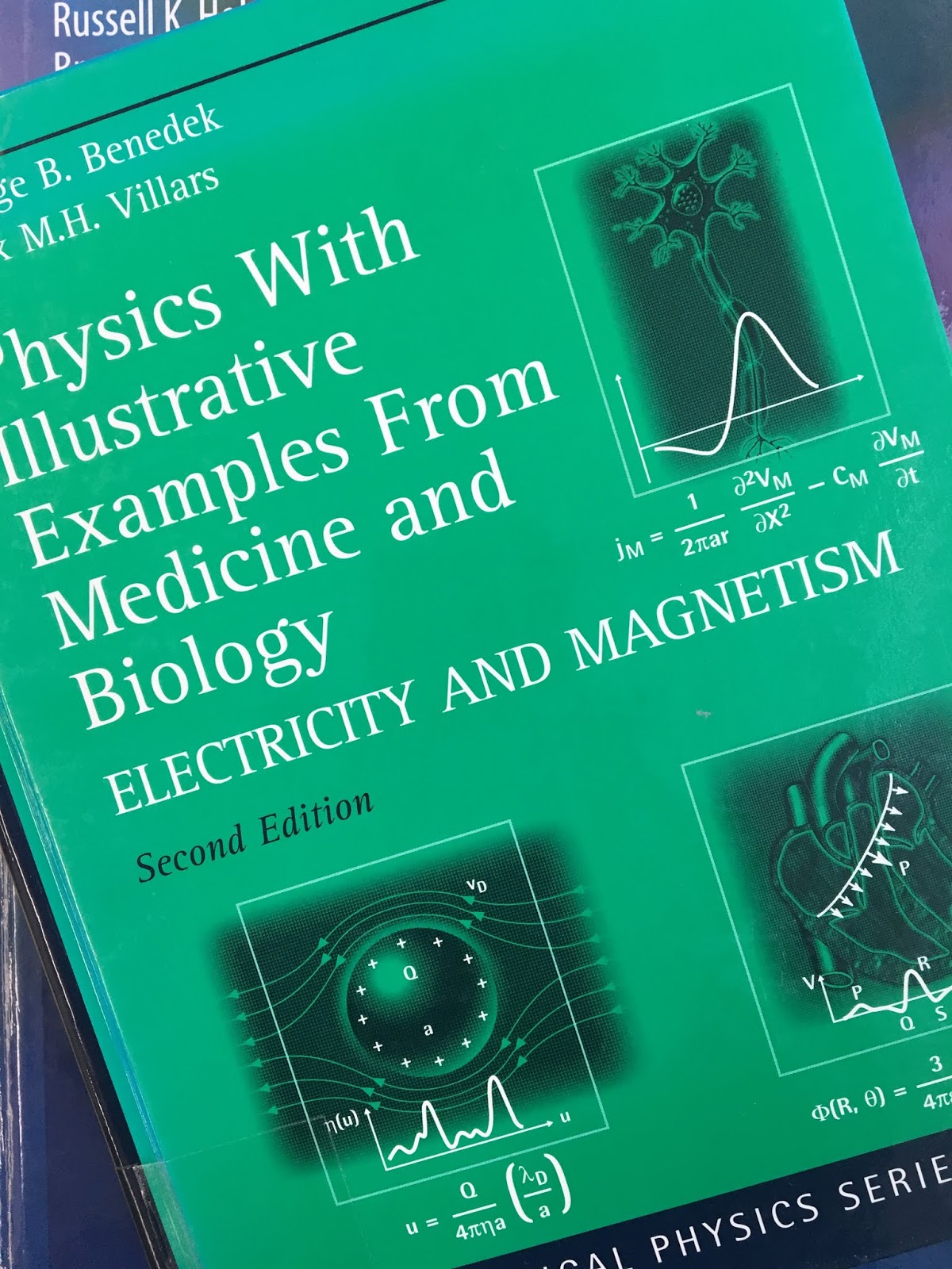
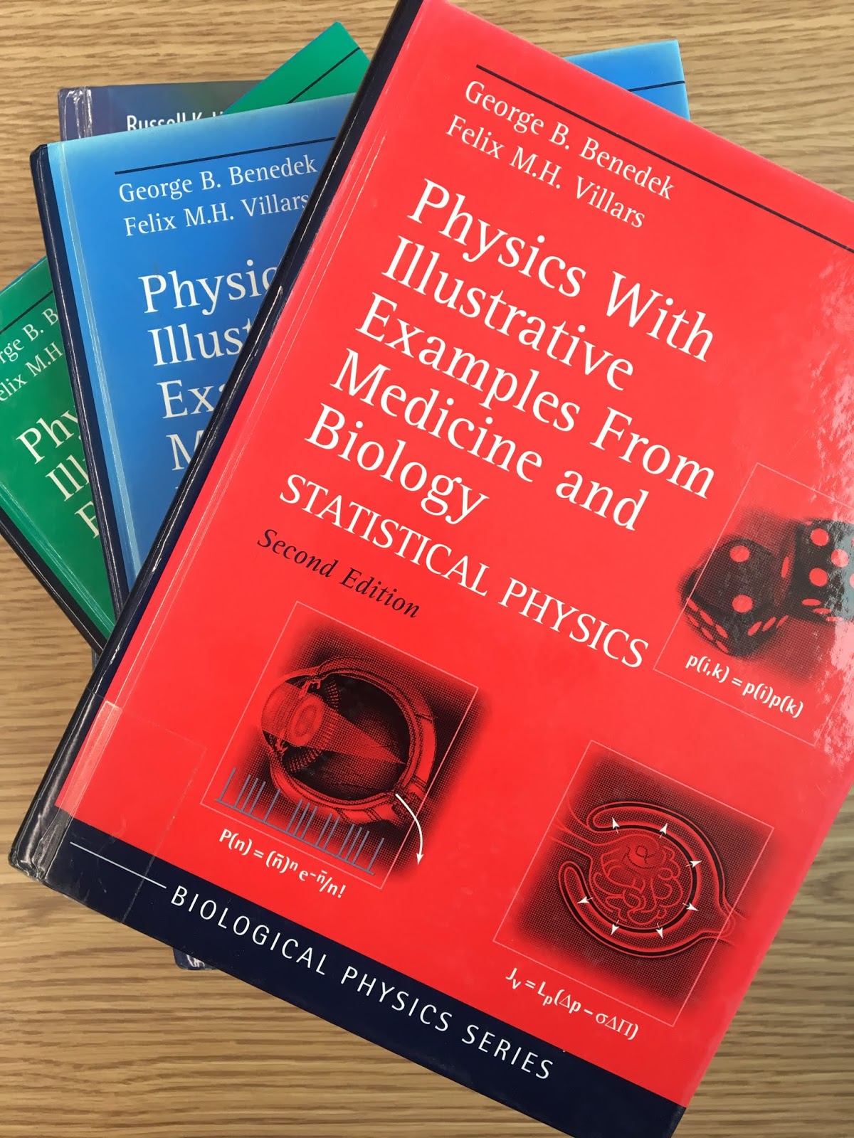
With this volume on Electricity and Magnetism, we complete the third and final volume of our textbooks on Physics, with Illustrative Examples from Medicine and Biology. We believe that this volume is as unique as our previous books on Classical Mechanics (Vol. 1) and Statistical Physics (Vol. 2). Here, we continue our program of interweaving into the rigorous development of classical physics, an analysis and clarification of a wide variety of important phenomena in physical chemistry, biology, physiology, and medicine.
All three volumes of Physics With Illustrative Examples From Medicine and Biology,
by Benedek and Villars.
The topics covered in Volume 3 are similar to those Russ Hobbie and I discuss in Chapters 6-9 in the 4th edition of Intermediate Physics for Medicine and Biology. Because I do research in the fields of bioelectricity and biomagnetism, you might expect that this would be my favorite volume of the three, but it’s not. I don’t find that it contains as many rich and interesting biological examples. Yet it is a solid book, and contains much useful electricity and magnetism.
Physics With Illustrative Examples From Medicine and Biology,
by Benedek and Villars.
Before leaving this topic, I should say a few words about George Benedek and Felix Villars. Benedek is currently the Alfred H. Caspary Professor of Physics and Biological Physics in the Department of Physics in the Harvard-MIT Division of Health Sciences and Technology. His group’s research program “centers on phase transitions, self-assembly and aggregation of biological molecules. These phenomena are of biological and medical interest because phase separation, self-assembly and aggregation of biological molecules are known to play a central role in several human diseases such as cataract, Alzheimer's disease, and cholesterol gallstone formation.” Villars was born in Switzerland. In the late 1940s, he collaborated with Wolfgang Pauli, and developed Pauli-Villars regularization. He began work at the MIT in 1950, where he collaborated with Herman Feshbach and Victor Weisskopf. He became interested in the applications of physics to biology and medicine, and helped establish the Harvard-MIT Division of Health Sciences and Technology. He died in 2002 at the age of 81.
In the present volume we develop and present the ideas of statistical physics, of which statistical mechanics and thermodynamics are but one part. We seek to demonstrate to students, early in their career, the power, the broad range, and the astonishing usefulness of a probabilistic, non-deterministic view of the origin of a wide range of physical phenomena. By applying this approach analytically and quantitatively to problems such as: the size of random coil polymers; the diffusive flow of solutes across permeable membranes; the survival of bacteria after viral attack; the attachment of oxygen to the binding sites on the hemoglobin molecule; and the effect of solutes on the boiling point and vapor pressure of volatile solvents; we demonstrate that the probabilistic analysis of statistical physics provides a satisfying understanding of important phenomena in fields as diverse as physics, biology, medicine, physiology, and physical chemistry.
If a bacterial culture is brought into contact with bacteriophage virus particles, the viruses will attack the bacteria and kill them in a matter of hours. However, a small number of bacteria do survive the attack. These survivors will reproduce and pass on to their descendants their resistance to the virus. The form of resistance of the offspring of the surviving bacteria is that their surface does not adsorb the attacking virus. Bacterial strains can also be resistant to metabolic inhibitors, such as streptomycin, penicillin, and sulphonamide. If a bacterial culture is subjected to attack by these antibiotics, the resistant strain will emerge just as in the case of the phage resistant bacteria.
In the early 1940s, Luria and Delbruck were working on ‘mixed infection’ experiments in which the bacteriophage resistant strain of E. coli bacteria were used as indicators in studies they were making on T1 and T2 virus particles. Starting in the Fall of 1942, they began to put aside the mixed infection experiment and asked themselves: What is the origin of those resistant bacterial strains that they were using as indicators?
They go on to give a detailed description of how Poisson statistics were used by Luria and Delbruck to study mutations.
Russ Hobbie and I discuss the Poisson distribution in our Appendix J. The Poisson distribution is an approximation of the more familiar binomial distribution, applicable for large numbers and small probabilities. One can see how this distribution would be appropriate for Luria and Delbruick, who had large numbers of viruses and a small probability of a mutation.
Russ and I cite Volume 1 of Benedek and Villars’ text in our Chapter 1 on biomechanics. We draw the data for our Fig. 4.12 from Benedek and Villars’ Volume 2. We never cite their Volume 3, about electricity and magnetism, which I’ll discuss next week.
I am an emeritus professor of physics at Oakland University, and coauthor of the textbook Intermediate Physics for Medicine and Biology. The purpose of this blog is specifically to support and promote my textbook, and in general to illustrate applications of physics to medicine and biology.


