Showing posts with label Lots of math. Show all posts

Friday, February 15, 2019

The Electric Field Induced During Magnetic Stimulation

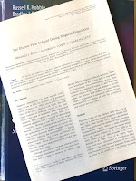
Chapter 8 of Intermediate Physics for Medicine and Biology discusses electromagnetic induction and magnetic stimulation of nerves. It doesn't, however, explain how to calculate the electric field. You can learn how to do this from my article “The Electric Field Induced During Magnetic Stimulation” (Electroencephalography and Clinical Neurophysiology, Supplement 43, Pages 268-278, 1991). It begins:
A photograph of the first page of The Electric Field Induced During Magnetic Stimulation by Roth, Cohen ad Hallett (EEG Suppl 43:268-278, 1991), superimposed on the cover of Intermediate Physics for Medicine and Biology.
“The Electric Field Induced
During Magnetic Stimulation.”
Magnetic stimulation has been studied widely since its use in 1982 for stimulation of peripheral nerves (Polson et al. 1982), and in 1985 for stimulation of the cortex (Barker et al. 1985). The technique consists of inducing current in the body by Faraday’s law of induction: a time-dependent magnetic field produces an electric field. The transient magnetic field is created by discharging a capacitor through a coil held near the target neuron. Magnetic stimulation has potential clinical applications for the diagnosis of central nervous system disorders such as multiple sclerosis, and for monitoring the corticospinal tract during spinal cord surgery (for review, see Hallett and Cohen 1989). When activating the cortex transcranially, magnetic stimulation is less painful than electrical stimulation.
Appendix 1 in the paper The Electric Field Induced During Magnetic Stimulation by Roth, Cohen ad Hallett (Electroencephalography and Clinical Neurophysiology, Suppl 43: 268-278, 1991), superimposed on the cover of Intermediate Physics for Medicine and Biology.
Appendix 1.
Although there have been many clinical studies of magnetic stimulation, until recently there have been few attempts to measure or calculate the electric field distribution induced in tissue. However, knowledge of the electric field is important for determining where stimulation occurs, how localized the stimulated region is, and what the relative efficacy of different coil designs is. In this paper, the electric field induced in tissue during magnetic stimulation is calculated, and results are presented for stimulation of both the peripheral and central nervous systems.
In Appendix 1 of this article, I derived an expression for the electric field E at position r, starting from
An equation for the electric field induced during magnetic stimulation.
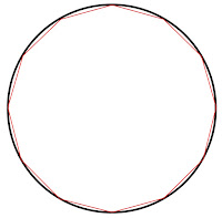
where N is the number of turns in the coil, μ0 is the permeability of free space (4π × 10-7 H/m), I is the coil current, r' is the position along the coil, and the integral of dl' is over the coil path. For all but the simplest of coil shapes this integral can't be evaluated analytically, so I used a trick: approximate the coil as a polygon. A twelve-sided polygon looks a lot like a circular coil. You can make the approximation even better by using more sides.
A circular coil approximated by a 12-sided polygon.
A circular coil (black) approximated by
a 12-sided polygon (red).
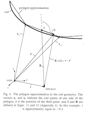
With this method I needed to calculate the electric field only from line segments. The calculation for one line segment is summarized in Figure 6 of the paper.
Figure 6 from The Electric Field Induced During Magnetic Stimulation, showing the polygon approximation to the coil geometry.
Figure 6 from “The Electric Field
Induced During Magnetic Stimulation.”
I will present the calculation as a new homework problem for IPMB. (Warning: t has two meanings in this problem: it denotes time and is also a dimensionless parameter specifying location along the line segment.)
Section 8.7

Problem 32 ½. Calculate the integral
The integral needed to calculate the electric field induced during magnetic stimulation.
for a line segment extending from x2 to x1. Define δ = x1 - x2 and R = r - ½(x1 + x2).
(a) Interpret δ and R physically.
(b) Define t as a dimensionless parameter ranging from -½ to ½. Show that r' equals rRtδ.
(c) Show that the integral becomes
An intermediate step in the calculation of the electric field induced during magnetic stimulation.
(d) Evaluate this integral. You may need a table of integrals.
(e) Express the integral in terms of δ, R, and φ (the angle between R and δ).

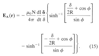
The resulting expression for the electric field is Equation 15 in the article
Equation (15) in The Electric Field During Magnetic Stimulation by Roth, Cohen ad Hallett (Electroencephalography and Clinical Neurophysiology, Suppl 43: 268-278, 1991).
Equation (15) in “The Electric Field Induced During Magnetic Stimulation.”
The photograph below shows the preliminary result in my research notebook from when I worked at the National Institutes of Health. I didn't save the reams of scrap paper needed to derive this result.

The November 10, 1988 entry in my research notebook, where I derive the equation for the electric field induced during magnetic stimulation.
The November 10, 1988 entry
in my research notebook.
To determine the ends of the line segments, I took an x-ray of a coil and digitized points on it. Below are coordinates for a figure-of-eight coil, often used during magnetic stimulation. The method was low-tech and imprecise, but it worked.

The November 17, 1988 entry in my research notebook, in which I digitized points along a figure-of-eight coil used for magnetic stimulation.
The November 17, 1988 entry
in my research notebook.
Ten comments:
  • My coauthors were Leo Cohen and Mark Hallett, two neurologists at NIH. I recommend their four-page paper “Magnetism: A New Method for Stimulation of Nerve and Brain.”
  • The calculation above gives the electric field in an unbounded, homogeneous tissue. The article also analyzes the effect of tissue boundaries on the electric field.
  • The integral is dimensionless. “For distances from the coil that are similar to the coil size, this integral is approximately equal to one, so a rule of thumb for determining the order of magnitude of E is 0.1 N dI/dt, where dI/dt has units of A/μsec and E is in V/m.”
  • The inverse hyperbolic sine can be expressed in terms of logarithms: sinh-1z = ln[z + √(z2 + 1)]. If you're uncomfortable with hyperbolic functions, perhaps logarithms are more to your taste. 
  • This supplement to Electroencephalography and Clinical Neurophysiology contained papers from the International Motor Evoked Potential Symposium, held in Chicago in August 1989. This excellent meeting guided my subsequent research into magnetic stimulation. The supplement was published as a book: Magnetic Motor Stimulation: Principles and Clinical Experience, edited by Walter Levy, Roger Cracco, Tony Barker, and John Rothwell
  • Leo Cohen was first author on a clinical paper published in the same supplement: Cohen, Bandinelli, Topka, Fuhr, Roth, and Hallett (1991) “Topographic Maps of Human Motor Cortex in Normal and Pathological Conditions: Mirror Movements, Amputations and Spinal Cord Injuries.”
  • To be successful in science you must be in the right place at the right time. I was lucky to arrive at NIH as a young physicist in 1988—soon after magnetic stimulation was invented—and to have two neurologists using the new technique on their patients and looking for a collaborator to calculate electric fields.
  • A week after deriving the expression for the electric field, I found a similar expression for the magnetic field. It was never published. Let me know if you need it.
  • If you look up my article, please forgive the incorrect units for μ0 given in the Appendix. They should be Henry/meter, not Farad/meter. In my defense, I had it correct in the body of the article. 
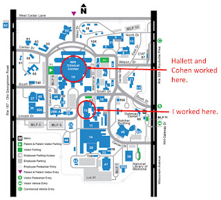
  • Correspondence about the article was to be sent to “Bradley J. Roth, Building 13, Room 3W13, National Institutes of Health, Bethesda, MD 20892.” This was my office when I worked at the NIH intramural program between 1988 and 1995. I loved working at NIH as part of the Biomedical Engineering and Instrumentation Program, which consisted of physicists, mathematicians and engineers who collaborated with the medical doctors and biologists. Cohen and Hallett had their laboratory in the NIH Clinical Center (Building 10), and were part of the National Institute of Neurological Disorders and Stroke. Hallett once told me he began his undergraduate education as a physics major, but switched to medicine after one of his professors tried to explain how magnetic fields are related to electric fields in special relativity.
A map of the National Institutes of Health campus in Bethesda, Maryland. I worked in Building 13. Hallett and Cohen worked in Building 10 (the NIH Clinical Center).
A map of the National Institutes of Health campus
in Bethesda, Maryland.

Friday, January 18, 2019

Five New Homework Problems About Diffusion

Diffusion is a central concept in biological physics, but it's seldom taught in physics classes. Russ Hobbie and I cover diffusion in Chapter 4 of Intermediate Physics for Medicine and Biology.

The one-dimensional diffusion equation,
The diffusion equation.
is one of the “big threepartial differential equations. Few analytical solutions to this equation exist. The best known is the decaying Gaussian (Eq. 4.25 in IPMB). Another corresponds to when the concentration is initially constant for negative values of x and is zero for positive values of x (Eq. 4.75). This solution is written in terms of error functions, which are integrals of the Gaussian (Eq. 4.74). I wonder: are there other simple examples illustrating diffusion? Yes!

In this post, my goal is to present several new homework problems that provide a short course in the mathematics of diffusion. Some extend the solutions already included in IPMB, and some illustrate additional solutions. After reading each new problem, stop and try to solve it!

Section 4.13
Problem 48.1. Consider one-dimensional diffusion, starting with an initial concentration of C(x,0)=Co for x less than 0 and C(x,0)=0 for x greater than 0. The solution is given by Eq. 4.75
A solution to the diffusion equation containing an error function.
where erf is the error function.
(a) Show that for all times the concentration at x=0 is C0/2.
(b) Derive an expression for the flux density, j = -DC/∂x at x = 0. Plot j as a function of time. Interpret what this equation is saying physically. Note: 
The derivative of the error function equals 2 over pi times the Gaussian function.

Problem 48.2. Consider one-dimensional diffusion starting with an initial concentration of C(x,0)=Co for |x| less than L and 0 for |x| greater than L.
(a) Plot C(x,0), analogous to Fig. 4.20.
(b) Show that the solution
A solution to the diffusion equation containing two error functions.
obeys both the diffusion equation and the initial condition.
(c) Sketch a plot of C(x,t) versus x for several times, analogous to Fig. 4.22.
(d) Derive an expression for how the concentration at the center changes with time, C(0,t). Plot it.

Problem 48.3. Consider one-dimensional diffusion in the region of x between -L and L. The concentration is zero at the ends, CL,t)=0.
(a) If the initial concentration is constant, C(x,0)=Co, this problem cannot be solved in closed form and requires Fourier series introduced in Chapter 11. However, often such a problem can be simplified using dimensionless variables. Define X = x/L, T = t/(L2/D) and Y = C/Co. Write the diffusion equation, initial condition, and boundary conditions in terms of these dimensionless variables.
(b) Using these dimensionless variables, consider a different initial concentration Y(X,0)=cos(Xπ/2). This problem has an analytical solution (see Problem 25). Show that Y(X,T)=cos(Xπ/2) e2T/4 obeys the diffusion equation as well as the boundary and initial conditions.

Problem 48.4. In spherical coordinates, the diffusion equation (when the concentration depends only on the radial coordinate r) is (Appendix L)

The diffusion equation in spherical coordinates.
Let C(r,t) = u(r,t)/r. Determine a partial differential equation governing u(r,t). Explain how you can find solutions in spherical coordinates from solutions of analogous one-dimensional problems in Cartesian coordinates.

Problem 48.5. Consider diffusion in one-dimension from x = 0 to ∞. At the origin the concentration oscillates with angular frequency ω, C(0,t) = Co sin(ωt).
(a) Determine the value of λ that ensures the expression
The solution to the diffusion equation when the concentration at the origin oscillates sinusoidally.
obeys the diffusion equation.
(b) Show that the solution in part (a) obeys the boundary condition at x = 0.
(c) Use a trigonometric identity to write the solution as the product of a decaying exponential and a traveling wave (see Section 13.2). Determine the wave speed.
(d) Plot C(x,t) as a function of x at times t = 0, π/2ω, π/ω, 3π/2ω, and 2π/ω.
(e) Describe in words how this solution behaves. How does it change as you increase the frequency?

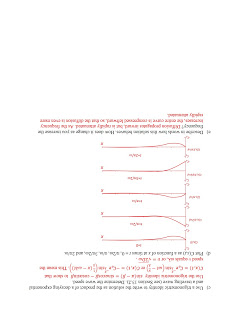
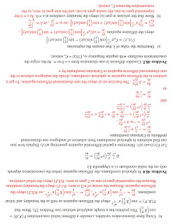
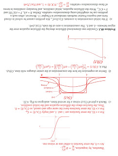
Of the five problems, my favorite is the last one; be sure to try it. But all the problems provide valuable insight. That’s why we include problems in IPMB, and why you should do them. I have included the solutions to these problems at the bottom of this post (upside down, making it more difficult to check my solutions without you trying to solve the problems first).

Random Walks in Biology, by Howard Berg, superimposed on the cover of Intermediate Physics for Medicine and Biology
Random Walks in Biology,
by Howard Berg.
Interested in learning more about diffusion? I suggest starting with Howard Berg’s book Random Walks in Biology. It is at a level similar to Intermediate Physics for Medicine and Biology.

After you have mastered it, move on to the classic texts by Crank (The Mathematics of Diffusion) and Carslaw and Jaeger (Conduction of Heat in Solids). These books are technical and contain little or no biology. Mathephobes may not care for them. But if you’re trying to solve a tricky diffusion problem, they are the place to go.

Enjoy!


Title page of The Mathematics of Diffusion, by Crank, superimposed on the cover of Intermediate Physics for Medicine and Biology.
The Mathematics of Diffusion.
The title page of Conduction of Heat in Solids, by Carslaw and Jaeger, superimposed on the cover of Intermediate Physics for Medicine and Biology.
The Conduction of Heat in Solids.
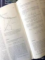
Page 45 of The Mathematics of Diffusion, by Crank. It contains a lot of equations.
I told you these books are technical! (Page 45 of Crank)
Page 4 of the solution to the new diffusion problems for Intermediate Physics for Medicine and Biology.
Page 4
Page 3 of the solution to the new diffusion problems for Intermediate Physics for Medicine and Biology.
Page 3
Page 2 of the solution to the new diffusion problems for Intermediate Physics for Medicine and Biology.
Page 2
Page 1 of the solution to the new diffusion problems for Intermediate Physics for Medicine and Biology.
Page 1

Friday, August 10, 2018

Craps

Intermediate Physics for Medicine and Biology
Intermediate Physics for Medicine and Biology.
This week I spent three days in Las Vegas.

I know you’ll be shocked...shocked!...to hear there is gambling going on in Vegas. If you want to improve your odds of winning, you need to understand probability. Russ Hobbie and I discuss probability in Intermediate Physics for Medicine and Biology. The most engaging way to introduce the subject is through analyzing games of chance. I like to choose a game that is complicated enough to be interesting, but simple enough to explain in one class. A particularly useful game for teaching probability is craps.

The rules: Throw two dice. If you role a seven or eleven you win. If you role a two, three, or twelve you lose. If you role anything else you keep rolling until you either “make your point” (get the same number that you originally rolled) and win, or “crap out” (roll a seven) and lose.

Two laws are critical for any probability calculation.
  1. For independent events, the probability of both event A and event B occurring is the product of the individual probabilities: P(A and B) = P(A) P(B).
  2. For mutually exclusive events, the probability of either event A or event B occurring is the sum of the individual probabilities: P(A or B) = P(A) + P(B).
Snake eyes
Snake Eyes.
For instance, if you roll a single die, the probability of getting a one is 1/6. If you roll two dice (independent events), the probability of getting a one on the first die and a one on the second (snake eyes) is (1/6) (1/6) = 1/36. If you roll just one die, the probability of getting either a one or a two (mutually exclusive events) is 1/6 + 1/6 = 1/3. Sometimes these laws operate together. For instance, what are the odds of rolling a seven with two dice? There are six ways to do it: roll a one on the first die and a six on the second die (1,6), or (2,5), or (3,4), or (4,3), or (5,2), or (6,1). Each way has a probability of 1/36 (the two dice are independent) and the six ways are mutually exclusive, so the probability of a seven is 1/36 + 1/36 + 1/36 + 1/36 + 1/36 + 1/36 = 6/36 = 1/6.

Boxcars
Boxcars.
Now lets analyze craps. The probability of winning immediately is 6/36 for a seven plus 2/36 for an eleven (a five and a six, or a six and a five), for a total of 8/36 = 2/9 = 22%. The probability of losing immediately is 1/36 for a two, plus 2/36 for a three, plus 1/36 for a twelve (boxcars), for a total of 4/36 = 1/9 = 11%. The probability of continuing to roll is….we could work it out, but the sum of the probabilities must equal 1 so a shortcut is to just calculate 1 – 2/9 – 1/9 = 6/9 = 2/3 = 67%.

The case when you continue rolling gets interesting. For each additional roll, you have three possibilities:
  1. Make you point and win with probability a
  2. Crap out and lose with probability b, or 
  3. Roll again with probability c.
What is the probability that, if you keep rolling, you make your point before crapping out? You could make your point on the first additional roll with probability a; you could roll once and then roll again and make your point on the second additional roll with probability ca; you could have three additional rolls and make your point on the third one with probability cca, etc. The total probability of making your point is a + ca + cca + … = a (1 + c + c2 + …). The quantity in parentheses is the geometric series, and can be evaluated in closed form: 1 + c + c2 + … = 1/(1 - c). The probability of making your point is therefore a/(1 - c). We know that one of the three outcomes must occur, so a + b + c = 1 and the odds of making your point can be expressed equivalently as a/(a + b). If your original roll was a four, then a = 3/36. The chance of getting a seven is b = 6/36. So, a/(a + b) = 3/9 = 1/3 or 33%. If your original roll was a five, then a = 4/36 and the odds of making your point is 4/10 = 40%. If your original roll was a six, the likelihood of making your point is 5/11 = 45%. You can work out the probabilities for 8, 9, and 10, but you’ll find they are the same as for 6, 5, and 4.

Now we have all we need to determine the probability of winning at craps. We have a 2/9 chance of rolling a seven or eleven immediately, plus a 3/36 chance of rolling a four originally followed by the odds of making your point of 1/3, plus…I will just show it as an equation.

P(winning) = 2/9 + 2 [ (3/36) (1/3) + (4/36) (4/10) + (5/36) (5/11) ] = 49.3 % .

The probability of losing would be difficult to work out from first principles, but we can take the easy route and calculate P(losing) = 1 – P(winning) = 50.7 %.

The chance of winning is almost even, but not quite. The odds are stacked slightly against you. If you play long enough, you will almost certainly lose on average. That is how casinos in Las Vegas make their money. The odds are close enough to 50-50 that players have a decent chance of coming out ahead after a few games, which makes them willing to play. But when averaged over thousands of players every day, the casino always wins.

Lady Luck, by Warren Weaver
Lady Luck, by Warren Weaver.
I hope this analysis helps you better understand probability. Once you master the basic rules, you can calculate other quantities more relevant to biological physics, such as temperature, entropy, and the Boltzmann factor (for more, see Chapter 3 of IPMB). When I teach statistical thermodynamics or quantum mechanics, I analyze craps on the first day of class. I arrive early and kneel in a corner of the room, throwing dice against the wall. As students come in, I invite them over for a game. It's a little creepy, but by the time class begins the students know the rules and are ready to start calculating. If you want to learn more about probability (including a nice description of craps), I recommend Lady Luck by Warren Weaver.

I stayed away from the craps table in Vegas. The game is fast paced and there are complicated side bets you can make along the way that we did not consider. Instead, I opted for blackjack, where I turned $20 into $60 and then quit. I did not play the slot machines, which are random number generators with flashing lights, bells, and whistles attached. I am told they have worse odds than blackjack or craps.

The trip to Las Vegas was an adventure. My daughter Stephanie turned 30 on the trip (happy birthday!) and acted as our tour guide. We stuffed ourselves at one of the buffets, wandered about Caesar’s Palace, and saw the dancing fountains in front of the Bellagio. The show Tenors of Rock at Harrah's was fantastic. We did some other stuff too, but let’s not go into that (What Happens in Vegas stays in Vegas).
A giant flamingo at the Flamingo
A giant flamingo at the Flamingo.
The High Roller Observation Wheel
The High Roller Observation Wheel.
Two Pina Coladas, one for each hand
Two Pina Coladas, one for each hand.

Friday, August 3, 2018

The Fourier Series of the Cotangent Function

In Section 11.5 of Intermediate Physics for Medicine and Biology, Russ Hobbie and I describe the Fourier series. I’m always looking for illustrative examples of Fourier series to assign as homework (see Problems 10.20 and 10.21), to explain in class, or to include on an exam. Not every function will work; it must be well behaved (in technical jargon, it must obey the Dirichlet conditions). Sometimes, however, I like to examine a case that does not satisfy these conditions, just to see what happens.

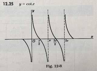
Consider the Fourier series for the cotangent function, cot(x) = cos(x)/sin(x).
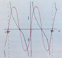
The cotangent function, from Schaum's Outlines: Mathematical Handbook of Formulas and Tables.

The function is periodic with period π, but at zero it asymptotically approaches infinity. Its Fourier series is defined as

The Fourier series written as a sum of sines (a's) and cosines (b's), of different frequencies.

where
The DC terms of the Fourier series, which is the average of the function.
The n'th coefficient a_n, an integral of the function times the cosine, for different frequencies.
The n'th coefficient b_n, an integral of the function times the sine, for different frequencies.

The cotangent is odd, implying that only sines contribute to the sum and a0 = an = 0. Because the product of two odd functions is even, we can change the lower limit of the integral for bn to zero and multiply the integral by two

The n'th coefficient b_n, an integral of cotangent times the sine, for different frequencies, integrated from zero to pi/2.

To evaluate this integral, I looked in the best integral table in the world (Gradshteyn and Ryzhik) and found

From Gradshteyn and Ryzhik: The integral of cot(x) times sin(2nx) is pi/2.

implying that bn = 2, independent of n. The Fourier series of the cotangent is therefore

cotangent written as a sum of 2 times sin(2x) plus 2 times sin(4x) plus 2 times sin(6x) and so on.

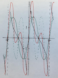
When I teach Fourier series, I require that students plot the function using just a few terms in the sum, so they can gain intuition about how the function is built from several frequencies. The first plot shows only the first term (red). It's not a good approximation to the cotangent (black), but what can you expect from a single frequency?
The cotangent function approximated by a single frequency.
The second plot shows the first term (green, solid), the second term (green dashed), and their sum (red). It’s better, but still has a long ways to go.

The cotangent function approximated by two frequencies.
If you add lots of frequencies the fit resembles the third plot (red, first ten terms). The oscillations don’t seem to converge to the function and their amplitude remains large.

The cotangent function approximated by ten frequencies.
The Youtube video below shows that the oscillation amplitude never dies down. It is like the Gibbs phenomenon on steroids; instead of narrow spikes near a discontinuity you get large oscillations everywhere.

The bottom line: the Fourier method fails for the cotangent; its Fourier series doesn’t converge. High frequencies contribute as much as low ones, and there are more of them (infinitely more). Nevertheless, we do gain insight by analyzing this case. The method fails in a benign enough way to be instructive.

I hope this analysis of a function that does not have a Fourier series helps you understand better functions that do. Enjoy!

Friday, July 27, 2018

Extrema of the Sinc Function

Intermediate Physics for Medicine and Biology: Extrema of the Sinc Function In Intermediate Physics for Medicine and Biology, Russ Hobbie and I write
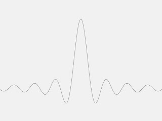
The function sin(x)/x has its maximum value of 1 at x = 0. It is also called the sinc(x) function.
Sinc(x) oscillates like sin(x), but its amplitude decays as 1/x. If sin(x) is zero then sinc(x) is also zero, except for the special point x = 0, where 0/0 becomes 1.
A plot of the sinc function
A plot of the sinc function.
Trigonomentric Delights  by Eli Maor
Trigonometric Delights, by Eli Maor
In IPMB, Russ and I dont evaluate the values of x corresponding to local maximum and minimum values of sinc(x). Eli Maor examines the peak values of f(x) = sinc(x) in his book Trigonometric Delights. He writes
We now wish to locate the extreme points of f(x)—the points where it assumes its maximum or minimum values. And here a surprise is awaiting us. We know that the extreme points of g(x) = sinx occur at all odd multiples of π/2, that is, at x = (2n+1)π/2. So we might expect the same to be true for the extreme points of f(x) = (sinx)/x. This, however, is not the case. To find the extreme point, we differentiate f(x) using the quotient rule and equate the result to zero:

          f’(x) = (x cosx – sinx)/x2 = 0.         (1)

Now if a ratio is equal to zero, then the numerator itself must equal to zero, so we have x cosx – sinx = 0, from which we get

          tan x = x.                                         (2)

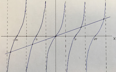
Equation (2) cannot be solved by a closed formula in the same manner as, say, a quadratic equation can; it is a transcendental equation whose roots can be found graphically as the points of intersection of the graphs of y = x and y = tan x.
Plots of y=x and y=tan(x), showing where they intersect
A plot of y=tanx versus x and y=x versus x.

The extreme values are at x = 0, 4.49 = 1.43π, 7.73 = 2.46π, etc. As x becomes large, the roots approach (2n+1)π/2.

Books by Eli Maor, including e, The Story of a Number
Eli Maor is a rare breed: a writer of mathematics. Russ and I cite his wonderful book e, The Story of a Number in Chapter 2 of IPMB. I also enjoyed The Pythagorean Theorem: A 4,000-year History. Maor has written many books about math and science. His most recent came out in May: Music by the Numbers--From Pythagoras to Schoenberg. I put it on my summer reading list.

Friday, April 27, 2018

Frequency Encoding and Phase Encoding

Intermediate Physics for Medicine and Biology: Frequency Encoding and Phase Encoding
I’m always searching for ways to illustrate concepts using “simple” analytical examples (I’ll let you decide whether or not this example is simple). Today, I present analytical examples of frequency and phase encoding during magnetic resonance imaging. Russ Hobbie and I discuss MRI in Chapter 18 of Intermediate Physics for Medicine and Biology.


1. Introduction

Our goal is to understand how the measured MRI signal changes when magnetic field gradients are present. These gradients are essential for “encoding” information about the spatial distribution of spins in the frequency and phase of the signal. To simplify our discussion, we make several assumptions:
  • The radio-frequency π/2 and π pulses, used to rotate the spins into the x-y plane and then create an echo, are so brief that the spins rotate instantaneously compared to all other time scales. Similarly, any slice selection gradient Gz = dBz/dz exists only during the radio-frequency pulses. We won’t include Gz in our drawings of pulse sequences. 
  • We ignore relaxation, so the longitudinal and transverse time constants T1 and T2 are infinite.
  • Despite ignoring relaxation, the spins do dephase leading to a free induction decay with time constant T2*. Dephasing is caused by a distribution of spin frequencies, corresponding to small-scale static heterogeneities of the magnetic field. We assume that the spin frequencies ω have the distribution
    The spin frequency distribution in an example of frequency encoding and phase encoding for magnetic resonance imaging.
    The peak frequency ωo is the Larmor frequency equal to γBo, where γ is the gyromagnetic ratio and Bo is the main magnetic field. The time constant τ indicates the width of the frequency distribution.

    A plot of the spin frequency distribution in an example of frequency encoding and phase encoding for magnetic resonance imaging.
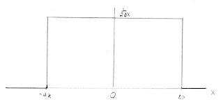
  • The spins are distributed uniformly along the x axis from -Δx to +Δx.
    A plot of the spin distribution in an example of frequency encoding and phase encoding for magnetic resonance imaging.

2. Spin-Echo

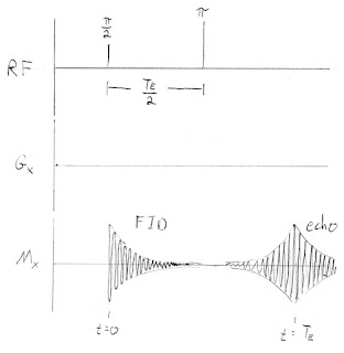
The spin-echo pulse sequence, with no gradients and no frequency or phase encoding, is similar to Fig. 18.24 in IPMB. Our pulse sequences consist of three functions of time. The radio-frequency (RF) pulses are shown on the first line; the time between the π/2 and π pulses is TE/2. The magnetic field gradient in the x direction, Gx = dBz/dx, is indicated in the second line; for this first example Gx is zero. The recorded signal, Mx, is in the third line.
MRI Spin-echo pulse sequence
Our goal is to calculate Mx(t). During the time between the two radio frequency pulses, we calculate the signal by integrating the precessing spins over x and ω

An integral giving the free induction decay during magnetic resonance imaging.

In this case the x integral is trivial: the integrand does not depend on x. We can solve the ω integral analytically using the u-substitution u=τ(ω-ωo), the cosine addition formula cos(A+B) = cosA cosB – sinA sinB, and the definite integral
A definite integral of cos(my)/(1+y^2)
The resulting free induction decay (FID) is

A mathematical expression for the free induction decay duing magnetic resonance imaging.
where τ corresponds to T2*. The exponential shape of the free induction decay arises from the particular form of our spin distribution. The wider the distribution of frequencies, the faster the decay.

The spins accumulate phase relative to those precessing at the Larmor frequency. Just before the π pulse the extra phase is (ω-ωo)TE/2. The π pulse changes the sign of this phase, or in other words adds an additional phase -(ω-ωo)TE. After the π pulse the signal is


The x integral is again trivial and the ω integral produces an echo


which peaks at t = TE and decays with time constant τ.

3. Phase Encoding

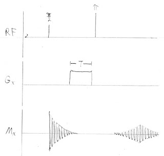
Phase encoding adds a gradient field Gx of duration T between the radio-frequency π/2 and π pulses. It shifts the phase of the spins by different amounts at different x locations (thus, position information is encoded in the phase of the signal). This phase shift is then reversed by the π pulse.
MRI phase encoding pulse sequence
The trickiest part of calculating Mx(t) is keeping track of the phase shifts: (ω-ωo)t is the phase shift up to time t because of the distribution of frequencies, -(ω-ωo)TE arises because the spins are flipped by the π pulse, γGxxT is caused by the phase-encoding gradient, and -2γGxxT is again from flipping by the π pulse. During the echo the signal simplifies to

An integral giving the echo during phase encoding in magnetic resonance imaging.

We can solve both the x and ω integrals by repeatedly using the cosine addition formula (it is tedious but not difficult; I leave the details to you), and find

A mathematical expression for the echo during phase encoding in magnetic resonance imaging.

The amplitude of the echo depends on the factor sin(γGxΔxT)/ (γGxΔxT). For a Gx of zero this factor is one and the result is the same as for the spin-echo. If we repeat this pulse sequence with different values of Gx and measure the amplitude of each echo, we can trace out the function sin(γGxΔxT)/ (γGxΔxT), which is the Fourier transform of the spin distribution as a function of position.

4. Frequency Encoding

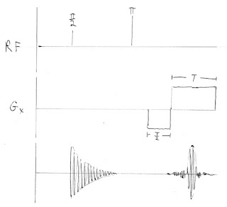
To do frequency encoding, we add a readout gradient Gx that is on during the echo and lasts a time T, like in Fig. 18.26 of IPMB. In addition, we include a prepulse of opposite polarity and half duration just before the readout, to cancel any extra phase shift accumulated during the echo. (Russ and I discuss this extra lobe of the Gx pulse when analyzing Fig. 18.29c, but we get its sign wrong).
MRI frequency encoding pulse sequence

The free induction decay and the phase reversal caused by the π-pulse are the same as in the spin-echo example. Once Gx begins the result differs. The frequency again depends on x. The phase shifts are: (ω-ωo)t because of the distribution of frequencies, -(ω-ωo)TE from the π pulse, -γGxxT/2 caused by the prepulse, and γGxx(t-(TE -T/2)) during readout. The recorded signal simplifies to

An integral giving the echo during frequency encoding during magnetic resonance imaging.

The echo during the readout gradient is (you really must fill in the missing steps yourself to benefit from this post)
The echo during frequency encoding during magnetic resonance imaging.
The envelope of the echo is the product of two terms, which are both functions of time: An exponential e-|t-TE|/τ that has the shape of the echo with no gradient, and a factor sin(γGxΔx(t-TE))/ (γGxΔx(t-TE)). The amplitude of the echo at t=TE is the same as if Gx were zero, but the shape of the echo has changed because of the time-dependent factor containing the gradient. The function containing the sine is the Fourier transform of the spin distribution. Therefore, the extra time-dependent modulation of the echo by Gx contains information about the spatial distribution of spins.

5. Conclusion

What do we learn from this example? A phase-encoding gradient changes the amplitude of the echo but not its shape. A frequency-encoding gradient, on the other hand, changes the shape but not the amplitude. Both can be written as a modulated Larmor-frequency signal. In the pulse sequences shown above, the Larmor frequency is drawn too low in order to make the figure clearer. In fact, the Larmor frequencies in MRI are many megahertz, and thousands of oscillations occur during the free induction decay and echo.

I analyzed both phase encoding and frequency encoding in the x direction and considered each individually, because I wanted to compare and contrast their behavior. In practice, frequency encoding is performed using a Gx gradient in the x direction and phase encoding with a Gy gradient in the y direction, mapping out the two-dimensional Fourier transform of the spin distribution (see IPMB for more). 

Until I did this calculation I never completely understood what the shape of the echo looks like during readout. I hope it helps you as much as it helped me. Enjoy!