Friday, January 25, 2013

Aliasing

In Chapter 11 of the 4th edition of Intermediate Physics for Medicine and Biology, Russ Hobbie and I discuss aliasing.
If a component [in the Fourier spectrum] is present whose frequency is more than half the sampling frequency, it will appear in the analysis at a lower frequency. This is the familiar stroboscopic effect in which the wheels of the stagecoach appear to rotate backward because the samples (movie frames) are not made rapidly enough. In signal analysis, this is called aliasing. It can be seen in Fig. 11.15, which shows a sine wave sampled at regularly spaced intervals that are longer than half a period.
First of all, what is all this business about a stagecoach? Fifty years ago, when westerns were all the rage in movies and on TV, aliasing often occurred if the frame rate (typically 24 frames per second for old movies) was lower than the rotation rate of the wheel (if all the spokes of the wheel are equivalent, then you can take the “period of rotation” as the time it takes for one spoke to rotate to the position of the adjacent one, which may be much shorter than the time for the wheel to make one complete rotation). You can see an example of this in the John Wayne movie Winds of the Wasteland (1936), especially in the climactic scene of the stagecoach race. In this video of the movie, you can see aliasing of the stagecoach wheel briefly at time 55:40. For those of you who are more discriminating in your movie tastes, you can see another example of aliasing 14 minutes and 15 seconds into Stagecoach, a John Wayne classic from 1939 directed by John Ford. In my opinion, the greatest western is the John Ford masterpiece The Man Who Shot Liberty Valance. What more could you ask for than both John Wayne and Jimmy Stewart in the same production? You can see aliasing briefly when Stewart drives his buckboard out of Shinbone to practice his pistol shooting (without much success). Another time when you see a wheel rotate backwards in this movie does not involve aliasing; it is (Spoiler Alert!) after Stewart Wayne kills Valance (Lee Marvin), when Pompey (Woody Strode) takes the drunken Wayne to his ranch house where he backs up the buckboard (that was a joke….).

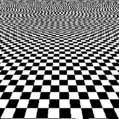
But I digress. Aliasing can happen in space as well as time, and can therefore affect images. If spatial frequencies in the structure of an object correspond to wavelengths smaller than the twice the pixel size, low spatial frequency artifacts, such as Moire patterns, can appear in the image, shown nicely in this figure. One can minimize aliasing by first filtering (anti-aliasing) before sampling. Some rather extreme cases of aliasing can been seen in Figs. 11.41 and 12.11 of Intermediate Physics for Medicine and Biology.

 Stagecoach, with John Wayne.

Friday, January 18, 2013

The Magic Angle

I recently found another error in the 4th edition of Intermediate Physics for Medicine and Biology. In Chapter 18 about magnetic resonance imaging, Homework Problem 18 reads
Problem 18  Suppose the two dipoles of the water molecule shown below point in the z direction while the line between them makes an angle θ with the x axis. Determine the angle θ for which the magnetic field of one dipole is perpendicular to the dipole moment of the other. For this angle the interaction energy is zero. This θ is called the “magic angle” and is used when studying anisotropic tissue such as cartilage [Xia (1998)].
Technically there is nothing wrong with this problem. However, if I were doing it over I would have the angle θ measured from the z axis, not the x axis. One reason is that this is the way θ is defined most often in the literature. Another is that in the solution manual we solve the problem as if θ were relative to the z axis, so the book and the solution manual are not consistent on the definition of θ. I should add, this problem was not present in the 3rd edition of Intermediate Physics for Medicine and Biology. It is a new problem I wrote for the 4th edition, so I can’t blame Russ Hobbie for this one (rats).

The citation in the homework problem is to the paper
Xia, Y. (1998) “Relaxation Anisotropy in Cartilage by NMR Microscopy (μMRI) at 14-μm Resolution,” Magnetic Resonance in Medicine, Volume 39, Pages 941–949.
The author, Yang Xia, is a good friend of mine, and a colleague here in the Department of Physics at Oakland University. He is well-known around OU because over the last decade he had the most grant money from the National Institutes of Health of anyone on campus. He uses a variety of techniques, including micro-magnetic resonance imaging (μMRI), to study cartilage and osteoarthritis. The abstract of his highly-cited paper reads
To study the structural anisotropy and the magic-angle effect in articular cartilage, T1 and T2 images were constructed at a series of orientations of cartilage specimens in the magnetic field by using NMR microscopy (μMRI). An isotropic T1, and a strong anisotropic T2 were observed across the cartilage tissue thickness. Three distinct regions in the microscopic MR images corresponded approximately to the superficial, transitional, and radial histological zones in the cartilage. The percentage decrease of T2 follows the pattern of the curve of (3cos2θ - 1)2 at the radial zone, where the collagen fibrils are perpendicular to the articular surface. In contrast, little orientational dependence of T2 was observed at the transitional zone, where the collagen fibrils are more randomly oriented. The result suggests that the interactions between water molecules and proteoglycans have a directional nature, which is somehow influenced by collagen fibril orientation. Hence, T2 anisotropy could serve as a sensitive and noninvasive marker for molecular-level orientations in articular cartilage.
Perhaps a better reference for our homework problem is another paper of Xia’s.
Xia, Y. (2000) “Magic Angle Effect in MRI of Articular Cartilage: A Review,” Investigative Radiology, Volume 35, Pages 602–621.
There in Fig. 3 of Xia’s review is a picture almost identical to the figure that immediately follows Homework Problem 18 in our book, except the angle θ is measured from the direction of the static magnetic field rather than perpendicular to it. Xia writes
T2 corresponds to the decay in phase coherence (dephasing) between the individual nuclear spins in a sample (protons in our case). Because each proton has a magnetic moment, it generates a small local dipolar magnetic field that impinges on its neighbor’s space (Fig. 3).43 This local field fluctuates constantly because the molecule is tumbling randomly. The T2 process can occur under the influence of this fluctuating magnetic field. At the end of signal excitation during an MRI experiment, the net magnetization (which produces the MRI signal) is coherent and points along a certain direction in space in the rotating frame of reference. This coherent magnetization vector soon becomes dephased because the local magnetic fields associated with the magnetic properties of neighboring nuclei cause the precessing nuclei to acquire a range of slightly different precessional frequencies. The time scale of this signal dephasing is reported as T2 and is characteristic of the molecular environment in the sample.43,44

For simple liquids or samples containing simple liquidlike molecules, the molecules tumble rapidly. The dipolar spin Hamiltonian (HD) that describes the dipolar interaction is averaged to zero, and its contribution to the spin relaxation vanishes. Relaxation characteristics exhibit a simple exponential decay that is well described by the Bloch equations.45 For samples containing molecules that are less mobile, HD is no longer averaged to zero and makes a significant contribution to the relaxation, resulting in a shorter T2. When HD is not zero, it is dominated by a geometric factor, (3cos2θ - 1), where θ is the angle between the position vector joining the two spins and the external magnetic field (see Fig. 3). A useful feature of this geometric factor is that it approaches zero as θ approaches 54.74° (Fig. 4). Therefore, even when HD is not zero, the contribution of HD to spin relaxation can be minimized if θ is set to 54.74°. This angle is called the magic angle in NMR.46
So, in the errata you will now find this:
Page 539: In Chapter 18, Homework Problem 18, “while the line between them makes an angle θ with the x axis” should be “while the line between them makes an angle θ with the z axis”. Also, in the accompanying figure following the homework problem, the angle θ should be measured from the z (vertical) axis, not the x (horizontal) axis. Corrected 1-18-13.
Is this the last error that we’ll find in our book? I doubt it; there are sure to be more we haven’t found yet. If you find any, please let us know.

Friday, January 11, 2013

5th Edition of Intermediate Physics for Medicine and Biology

Russ Hobbie and I are starting to talk about a 5th edition of Intermediate Physics for Medicine and Biology, and we need your help. We would like suggestions and advice about what changes/additions/deletions to make in the new edition.

We have prepared a survey to send to faculty members who we know have used IPMB as the textbook for a class they taught. However, our list may be incomplete, and input from any teacher, student, or reader would be useful. So, below is a copy of the survey. Please send responses to any or all of the questions to Russ (hobbie@umn.edu).

Thanks!
  1. What chapters did you cover when teaching from the 4th edition of IPMB?
  2. Were the homework problems appropriate?
  3. In the 4th edition we added a chapter on Sound and Ultrasound to IPMB. If we were to add one new chapter to the 5th edition, what should the topic be?
  4. Would color significantly improve the book for your purposes? How much extra money would you be willing to pay if the 5th edition contained many color pictures?
  5. What is the best feature of IPMB? What is the worst?
  6. Is the end-of-chapter list of symbols useful?
  7. Do your students use the Appendices? Suppose to save space one Appendix had to be deleted: which one should go?
  8. Did you have access to the solution manual? Was it useful? The solution manual we prepared using different software than the book itself. Did you see a noticeable difference in the quality of the book and the solution manual?
  9. Would you like students to have access to the solution manual?
  10. Did you use any information on the book website, such as the errata or text from previous editions?
  11. Are you aware of the book blog? Did you find it useful when teaching from IPMB? Do you find it interesting?
  12. How important is having a paperback version of the book?
  13. What textbooks did you consider other than IPMB? If IPMB did not exist, what book would you use for your class?

Friday, January 4, 2013

Non-Dynamical Stochastic Resonance: Theory and Experiments with White and Arbitrarily Coloured Noise

Section 11.18 of the 4th edition of Intermediate Physics for Medicine and Biology contains a discussion of stochastic resonance. This is a new section that Russ Hobbie and I added to the 4th edition, and features a discussion of a paper by Zoltan Gingl, Laszlo Kish (formerly “Kiss”), and Frank Moss.
Gingl, Z., L. B. Kiss, and F. Moss (1995) “Non-Dynamical Stochastic Resonance: Theory and Experiments with White and Arbitrarily Coloured Noise,” Europhysics Letters, Volume 29, Pages 191–196.
The paper is interesting (despite the annoying British spelling), and I reproduce part of the introduction below.
In the last decade’s physics literature, stochastic-resonance (SR) effect has been one of the most interesting phenomena taking place in noisy non-linear dynamical systems (see, e.g., [l-14]. The input of stochastic resonators [12] (non-linear systems showing SR) is fed by a Gaussian noise and a sinusoidal signal with frequency f0, that is, a random excitation and a periodic one are acting on the system. There is an optimal strength of the input noise, such that the system’s output power spectral density, at the signal frequency f0, has a maximal value. This effect is called SR. It can be viewed as: the transfer of the input sinusoidal signal through the system shows a “resonance vs. the strength of the input noise. It is a very interesting, and somewhat paradoxial effect, because it indicates that in these systems the existence of a certain amount of “indeterministic excitation is necessary to obtain the optimal “deterministic response. There are certain indications [2,13,14] that the principle of SR may be applied by nature in biological systems in order to optimise the transfer of neural signals.
Until last year, it was a common belief that SR phenomena occur only in (bistable, sometimes monostable [10] or multistable) dynamical systems [1-14]. Very recently, Wiesenfeld et al. [15] have proposed that certain systems with threshold-like properties should also show SR effects.
We present here an extremely simple system, invented by Moss, which displays SR. It consists only of a threshold and a subthreshold coherent signal plus noise as shown in fig. la). It is not a dynamical system, instead there is a single rule: whenever the signal plus the noise crosses the threshold unidirectionally, a narrow pulse of standard shape is written to a time series, as shown in fig. lb). The power spectrum of this series of pulses is shown in fig. 1c). It shows all the familiar features of SR systems previously studied [l, 2, 7, 16], in particular, the narrow, delta-like signal features riding on a broad-band noise background from which the signal-to-noise ratio (SNR) can be extracted. This system can be easily realized electronically as a level-crossing detector (LCD). There is a simple and very physically motivated theory of this phenomenon (due to Kiss), see below. Other, more detailed studies of various aspects of threshold-crossing dynamics have been made by Fox et al. [17], Jung [18] and Bulsara et al. [19].
We have experimentally realised and developed this simple SR system and carried out extensive analog and computer simulations on it. The theory of Kiss has been verified for the case of white and several sorts of coloured noises. Until now, the description of this new SR system, its physical realisation and the original theory have not appeared in the open literature, so in this letter we shall describe the new system and its developments made by us, present the outline and the main results of the theory and finally show some interesting experimental results…
Figure 1 in their paper is our Figure 11.50. It is an excellent figure, although I don’t know why they didn’t adjust the time axes so that the pulses in b) are aligned precisely with the signal crossings in a). The axes are almost correct, but are off just enough to be confusing, like when the video and audio signals are off by a fraction of a second in a movie or TV show.

The Gingl et al. paper is short and highly cited (over 200 citations to date, according to the Web of Science). However, it is not cited nearly as often as another paper published by Kurt Wisenfeld and Moss that same year:
Wisenfeld K. and F. Moss (1995) “Stochastic Resonance and the Benefits of Noise: From Ice Ages to Crayfish and SQUIDs,” Nature, Volume 373, Pages 33–36.
This paper, with over 1000 citations, reviews many applications of stochastic resonance.
Noise in dynamical systems is usually considered a nuisance. But in certain nonlinear systems, including electronic circuits and biological sensory apparatus, the presence of noise can in fact enhance the detection of weak signals. This phenomenon, called stochastic resonance, may find useful application in physical, technological and biomedical contexts.
Wisenfeld and Moss discuss how the crayfish may use stochastic resonance to detect weak signals with their mechanoreceptor hair cells.

Frank Moss (1934-2011) was the founding director of the Center for Neurodynamics at the University of Missouri at St Louis. Click here to read his obituary (he died two years ago today) in Physics Today, and click here to read a tribute to him in a focus issue of the journal Chaos.