Numerical Solution of the Quadratic Formula

Homework Problem 7 in Chapter 11 of Intermediate Physics for Medicine and Biology examines fitting data to a straight line. In that problem, the four data points to be fit are (100, 4004), (101, 4017), (102, 4039), and (103, 4063). The goal is to fit the data to the line y = ax + b. For this data, one must perform the calculation of a and b to high precision or else you get large errors. The solution manual (available to instructors upon request) says that

This problem illustrates how students can run into numerical problems if they are not careful. With modern calculators that carry many significant figures, this may seem like a moot point. But the idea is still important and can creep subtly into computer computations and cause unexpected, difficult-to-debug errors.

Numerical Recipes

Are there other examples of numerical errors creeping into calculations? Yes. You can find one discussed in Numerical Recipes that involves the quadratic formula.

We all know the quadratic formula from high school. If you have a quadratic equation of the form

the solution is

For example,
 

has two solutions
 

so x = 1 or 2.

Now, suppose the coefficient b is larger,

The solution is

so x = 300 or 0.00667.

This calculation is susceptible to numerical error. For instance, suppose all numerical calculations are performed to only four significant figures. Then when you reach the step

you must subtract 8 from 90,000. You get 89992, which to four significant figures becomes 89990, which has a square root of (again to four significant figures) 300.0. The solutions are therefore x = 300 or 0. The large solution (300) is correct, but the small solution (0 instead of 0.00667) is completely wrong. The main reason is that when using the minus sign for ± you must subtract two numbers that are almost the same (in this case, 300 – 299.98667) to get a much smaller number.

You might say “so what! Who uses only four significant figures in their calculations?” Okay, try solving

where I increased b from 300 to 3000. You’ll find that using even six significant figures gives one nonsense solution (try it). As you make b larger and larger, the calculation becomes more and more difficult. The situation can cause unexpected, difficult-to-debug errors.

What’s the moral to this story? Is it simply that you must use high precision when doing calculations? No. We can do better. Notice that the solution is fine when using the plus sign in the quadratic equation. We need make no changes. It’s the negative sign that gives the problem,
 

Let’s try a trick; multiply the expression by a very special form of one:

Simplifying, we get

Voilà! The denominator has the plus sign in front of the square root, so it is not susceptible to numerical error. The numerator is simplicity itself. Try solving x² – 300x + 2 = 0 using math to four significant figures,

 

No error, even with just four sig figs. The problem is fixed!

I should note that the problem is fixed only for negative values of b. If b is positive, you can use an analogous approach to get a slightly different form of the solution (I’ll leave that as an exercise for the reader).

So, the moral of the story is: if you find that your numerical calculation is susceptible to numerical error, fix it! Look for a trick that eliminates the problem. Often you can find one.

Stirling's Approximation

I've always been fascinated by Stirling’s approximation,

ln(n!) = n ln(n) − n,

where n! is the factorial. Russ Hobbie and I mention Stirling’s approximation in Appendix I of Intermediate Physics for Medicine and Biology. In the homework problems for that appendix (yes, IPMB does has homework problems in its appendices), a more accurate version of Stirling’s approximation is given as

ln(n!) = n ln(n) − n + ½ ln(2π n) .

There is one thing that’s always bothered me about Stirling’s approximation: it’s for the logarithm of the factorial, not the factorial itself. So today, I’ll derive an approximation for the factorial. 

The first step is easy; just apply the exponential function to the entire expression. Because the exponential is the inverse of the natural logarithm, you get

n! = e^{n ln(n) − n + ½ ln(2π n)}

Now, we just use some properties of exponents

n! = e^{n ln(n)} e⁻ⁿ e^{½ln(2π n)}

n! = (e^ln(n))ⁿ e⁻ⁿ √(e^{ln(2π n)})

n! = nⁿ e⁻ⁿ √(2π n) 

And there we have it. It’s a strange formula, with a really huge factor (nⁿ) multiplied by a tiny factor (e⁻ⁿ) times a plain old modestly sized factor (√(2π n)). It contains both e = 2.7183 and π = 3.1416.

Let's see how it works.

n	n!	nn e−n √(2π n)	fractional error (%)
1	1	0.92214	7.8
2	2	1.9190	4.1
5	120	118.02	1.7
10	3.6288 × 106	3.5987 × 106	0.83
20	2.4329 × 1018	2.4228 × 1018	0.42
50	3.0414 × 1064	3.0363 × 1064	0.17
100	9.3326 × 10157	9.3249 × 10157	0.083

For the last entry (n = 100), my calculator couldn’t calculate 100¹⁰⁰ or 100!. To get the first one I wrote

100¹⁰⁰ = (10²)¹⁰⁰ = 10^{2 × 100} = 10²⁰⁰.

The calculator was able to compute e⁻¹⁰⁰ = 3.7201 × 10⁻⁴⁴, and of course the square root of 200π was not a problem. To obtain the actual value of 100!, I just asked Google.

Why in the world does anyone need a way to calculate such big factorials? Russ and I use them in Chapter 3 about statistical dynamics. There you have to count the number of states, which often requires using factorials. The beauty of statistical mechanics is that you usually apply it to macroscopic systems with a large number of particles. And by large, I mean something like Avogadro’s number of particles (6 × 10²³). The interesting thing is that in statistical mechanics you often need not the factorial, but the logarithm of the factorial, so Stirling's approximation is exactly what you want. But it’s good to know that you can also approximate the factorial itself. 

Finally, one last fact from Mr. Google. 1,000,000! = 8.2639 × 10^5,565,708. Wow!

Stirling’s Approximation

https://www.youtube.com/watch?v=IJ5N28-Ujno

The Helmholtz Coil and the Maxwell Coil

To do magnetic resonance imaging, you need a static magnetic field that is uniform and a switchable magnetic field that has a uniform gradient. How do you produce such fields? In this post, I explain one of the simplest ways: using a Helmholtz coil and a Maxwell coil.

Both of these are created using circular coils. The magnetic field B_z produced by a circular coil can be calculated using the law of Biot and Savart (see Chapter 8 of Intermediate Physics for Medicine and Biology)

where μ₀ is the permeability of free space (the basic constant of magnetostatics), I is the coil current, N is the number of turns, R is the coil radius, and z is the distance along the axis from the coil center.

The Helmholtz Coil

The Helmholtz coil consists of two circular coils in parallel planes, having the same axis and the same current in the same direction, that are separated by a distance d. Our goal will be to find the value of d that gives the most uniform magnetic field. By superposition, the magnetic field is 

 

To create a uniform magnetic field, we will perform a Taylor expansion of the magnetic field about the origin (z = 0). We will need derivatives of the magnetic field. The first derivative is

(The reader will have to fill in the missing steps when calculating these derivatives.) At z = 0, this derivative will go to zero. In fact, because the magnetic field is even about the z axis, all odd derivatives will be zero, regardless of the value of d.

The second derivative is

At z = 0, the two terms in the brackets are the same. Our goal is to have this term be zero, implying that the second order term in the Taylor series vanishes. This will happen if

or, in other words, d = R. This famous result says that for a Helmholtz pair the coil separation should equal the coil radius.

A Helmholtz coil produces a remarkably uniform field near the origin. However, it is not uniform enough for use in most magnetic resonance imaging machines, which typically have a more complex set of coils to create an even more homogeneous field. If you need a larger region that is homogeneous, you could always just use a larger Helmholtz coil, but then you would need more current to achieve the desired magnetic field at the center. A Helmholtz pair isn’t bad if you want to use only two reasonably sized coils.

The Maxwell Coil

The Helmholtz coil produces a uniform magnetic field, whereas the Maxwell coil produces a uniform magnetic field gradient. It consists of two circular coils, in parallel planes having the same axis, that are separated by a distance d, but which have current in the opposite directions. Again, our goal will be to find the value of d that gives the most uniform magnetic field gradient. The magnetic field is

The only difference between this case and that for the Helmholtz coil is the change in sign of the second term in the bracket. If z = 0, the magnetic field is zero. Moreover, the magnetic field is an odd function of z, so all even derivatives also vanish. The first derivative is

This expression gives us the magnitude of the gradient at the origin, but it doesn’t help us create a more uniform gradient. The second derivative is

This derivative is zero at the origin, regardless of the value of d. So, we have to look at the third derivative.

At z = 0, this will vanish if

or, in other words, d = √3 R = 1.73 R. Thus, the two coils have a greater separation for a Maxwell coil than for a Helmholtz coil. The Maxwell coil would be useful for producing the slice selection gradient during MRI (for more about the need for gradient fields in MRI, see Chapter 18 of IPMB).

Conclusion

Below is a plot of the normalized magnetic field as a function of z for the Helmholtz coil (blue) and the Maxwell coil (yellow). As you can see, the region with a uniform field or gradient is small. It depends on what level of accuracy you need, but if you are more than half a radius from the origin you will see significant deviations from homogeneity.
 

Russ Hobbie and I never discuss the Helmholtz coil in Intermediate Physics for Medicine and Biology. We don’t mention the Maxwell coil by name, but Problem 33 of Chapter 18 analyzed a Maxwell pair even if we don’t call it that.

The Maxwell coil is great for producing the magnetic field gradient dB_z/dz needed for slice selection in MRI, but how do you produce the gradients dB_z/dx and dB_z/dy needed during MRI readout and phase encoding? That, my friends, is a story for another post.

Decay Plus Input at a Constant Rate Revisited

In Chapter 2 of Intermediate Physics for Medicine and Biology, Russ Hobbie and I discuss the problem of decay plus input at a constant rate.

Suppose that in addition to the removal of y from the system at a rate –by, y enters the system at a constant rate a, independent of y and t. The net rate of change of y is given by

Then we go on to discuss how you can learn things about a differential equation without actually solving it.

It is often easier to write down a differential equation describing a problem than it is to solve it… However, a good deal can be learned about the solution by examining the equation itself. Suppose that y(0) = 0. Then the equation at t = 0 is dy/dt = a, and y initially grows at a constant rate a. As y builds up, the rate of growth decreases from this value because of the –by term. Finally when a – by = 0, dy/dt is zero and y stops growing. This is enough information to make the sketch in Fig. 2.13.

The equation is solved in Appendix F. The solution is

… The solution does have the properties sketched in Fig. 2.13, as you can see from Fig. 2.14.

Figure 2.13 looks similar to this figure

Sketch of the initial slope a and final value a/b of y when y(0) = 0. In this figure, a=b=1.

 And Fig. 2.14 looks like this

A plot of y(t) using Eq. 2.26, with a=b=1.

However, Eq. 2.26 is not the only solution that is consistent with the sketch in Fig. 2.13. Today I want to present another function that is consistent with Fig. 2.13, but does not obey the differential equation in Eq. 2.25.

Let’s examine how this function behaves. When bt is much less than one, the function becomes y = at, so it’s initial growth rate is a. When bt is much greater than one, the function approaches a/b. The sketch in Fig. 2.13 is consistent with this behavior.

Below I show both Eqs. 2.26 and 2.26’ in the same plot.

A plot of y(t) using Eq. 2.26 (blue) and Eq. 2.26' (yellow), with a=b=1.

The function in Eq. 2.26 (blue) approaches its asymptotic value at large t more quickly than the function in Eq. 2.26’ (yellow).

The moral of the story is that you can learn a lot about the behavior of a solution by just inspecting the differential equation, but you can’t learn everything (or, at least, I can’t). To learn everything, you need to solve the differential equation. 

By the way, if Eq. 2.26’ doesn’t solve the differential equation in Eq. 2.25, then what differential equation does it solve? The answer is

 How did I figure that out? Trial and error.

A Short Course in Vector Calculus

Want a short course in vector calculus? You can find one in Intermediate Physics for Medicine and Biology.

Divergence

The divergence is defined in Section 4.1 in IPMB, when discussing the continuity equation. The divergence is one way to differentiate a vector field. I our case, the vector field is the current density (or some other type of flux density), j. Its divergence is defined as 

When you take the divergence of a vector (a quantity that has both magnitude and direction), you get a scalar (a quantity that has magnitude but no direction). In electrostatics, the electrical charge is conserved, implying that the divergence of the electrical current density is zero.

Curl

The curl is defined in Section 8.6, when analyzing electromagnetic induction. It is another way to differentiate a vector,

The symbols x̂, ŷ, and ẑ are unit vectors, and the vertical lines indicate that you follow the rules for determinants when expanding this expression. The curl appears often when analyzing the magnetic field. In our case, the curl of the electric field equations the negative of the time derivative of the magnetic field (Faraday’s law of induction).

Gradient

The gradient is a way to differentiate a scalar field to get a vector. 

 

You can think of the gradient, ∇, as representing the vector x̂ ∂/∂x + ŷ ∂/∂y + ẑ ∂/∂z. The divergence is then found by taking the dot product of the gradient with a vector, and the curl is found by taking the cross product of the gradient with the vector. In electrostatics, V represents of the electric potential (a scalar) and E represents the electric field (a vector). The two are related by

Laplacian

The Laplacian, ∇², is just the dot product of the gradient operator with itself. In other words 

 

You can apply the Laplacian to a vector, but it is more commonly applied to a scalar (such as electrical potential, temperature, or concentration). The Europeans use ∆ to represent the Laplacian, but that’s just weird and we Americans know better than that.

Other Coordinate Systems

We have written the divergence, curl, gradient, and Laplacian in Cartesian coordinates. These operators are more complicated in other coordinate systems. Appendix L of IPMB provides expressions for these operators in cylindrical coordinats of spherical coordinates.

The Divergence Theorem

The divergence theorem says that the volume integral of div J is equal to the surface integral of the normal component of J. We don’t dwell on this theorem in IPMB, but we do ask the reader to derive it in Homework Problem 4 of Chapter 4.

Stokes’ Theorem

We don’t discuss Stokes’ Theorem in IPMB, but I’ve pointed out how we might include a homework problem about it in a previous blog post. Stokes’ theorem says that the line integral of a vector around a closed loop is equal to the surface integral of the curl of that vector of an area bounded by the loop.

div, grad, curl, and all that,
by h. m. schey.

So, almost all the big concepts of vector calculus are presented in IPMB. If, however, you want a little more detail, Russ and I recommend the wonderful book div, grad, curl, and all that, by Harry Schey. I learned vector calculus from the first edition of that book as an undergraduate physics major at the University of Kansas. Schey died five years ago, but his book lives on.

Integral of the Bessel Function

Have you ever been reading a book, making good progress with everything making sense, and then you suddenly stop at say “wait… what?”. That happened to me recently as I was reading Homework Problem 31 in Chapter 12 of Intermediate Physics for Medicine and Biology. (Wait…what? I’m a coauthor of IPMB! How could there be any surprises for me?) The problem is about calculating the two-dimensional Fourier transform of 1/r, and it supplies the following Bessel function identity 

The function J₀ is a Bessel function of the first kind of order zero. What surprised me is that if you let x = kr, you get that the integral of the Bessel function is one,

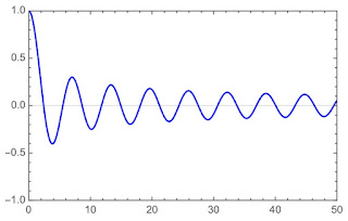
Really? Here’s a plot of J₀(x).

It oscillates like crazy and the envelope of those oscillations falls off very slowly. In fact, an asymptotic expansion for J₀ at large x is

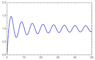
The leading factor of 1/√x decays so slowly that its integral from zero to infinity does not converge. Yet, when you include the cosine so the function oscillates, the integral does converge. Here’s a plot of

The integral approaches one at large x, but very slowly. So, the expression given in the problem is correct, but I sure wouldn’t want to do any numerical calculations using it, where I had to truncate the endpoint of the integral to something less than infinity. That would be a mess!

Here’s another interesting fact. Bessel functions come in many orders—J₀, J₁, J₂, etc.—and they all integrate to one.

Who’s responsible for these strangely-behaved functions? They’re named after the German astronomer Friedrich Bessel but they were first defined by the Swiss mathematician Daniel Bernoulli (1700–1782), a member of the brilliant Bernoulli family. The Bernoulli equation, mentioned in Chapter 1 of IPMB, is also named for Daniel Bernoulli. 

There was a time when I was in graduate school that I was obsessed with Bessel functions, especially modified Bessel functions that don’t oscillate. I’m not so preoccupied by them now, but they remain my favorite of the many special functions encountered in physics.

The Partition Function

Any good undergrad statistical mechanics class analyzes the partition function. However, Russ Hobbie and I don’t introduce the partition function in Intermediate Physics for Medicine and Biology. Why not? It’s a long story.

Russ and I do discuss the Boltzmann factor. Suppose you have a system that is in thermal equilibrium with a reservoir at absolute temperature T. Furthermore, suppose your system has discrete energy levels with energy E_i, where i is just an integer labeling the levels. The probability P_i of the system being in level i, is proportional to the Boltzmann factor, exp(–E_i/k_BT),

P_i = C exp(–E_i/k_BT),

where exp is the exponential function, k_B is the Boltzmann constant and C is a constant of proportionality. How do you find C? Any probability must be normalized: the sum of the probabilities must equal one,

Σ P_i = 1 ,

where Σ indicates a summation over all values of i. This means

Σ C exp(–E_i/k_BT) = 1,

or

C = 1/[Σ exp(–E_i/k_BT)] .

The sum in the denominator is the partition function, and is usually given the symbol Z,

Z = Σ exp(–E_i/k_BT) .

In terms of the partition function, the probability of being in state P_i is simply

P_i = (1/Z) exp(–E_i/k_BT) .

An Introduction to Thermal Physics,
by Daniel Schroeder.

Here is what Daniel Schroeder writes in his excellent textbook An Introduction to Thermal Physics,

The quantity Z is called the partition function, and turns out to be far more useful than I would have suspected. It is a “constant” in that it does not depend on any particular state s [he uses “s” rather than “i” to count states], but it does depend on temperature. To interpret it further, suppose once again that the ground state has energy zero. Then the Boltzmann factor for the ground state is 1, and the rest of the Boltzmann factors are less than 1, by a little or a lot, in proportion to the probabilities of the associated states. Thus, the partition function essentially counts how many states are accessible to the system, weighting each one in proportion to its probability.

To see why it’s so useful, let’s define β as 1/k_BT. The Boltzmann factor is then

exp(–βE_i)

and the partition function is

Z = Σ exp(–βE_i) .

The average energy, <E>, is

<E> = [Σ E_i exp(–βE_i)]/[Σ exp(–βE_i)] .

The denominator is just Z. The numerator can be written as the negative of the derivative of Z with respect to β, dZ/dβ (try it and see). So, the average energy is

<E> = – (1/Z) dZ/dβ .

I won’t go on, but there are other quantities that are similarly related to the partition function. It’s surprisingly useful.

Is the partition function hidden in IPMB? You might recognize it in Eq. 3.37, which determines the average kinetic energy of a particle at temperature T (the equipartition of energy theorem) It looks a little different, because there’s a continuous range of energy levels, so the sum is disguised as an integral. You can see it again in Eq. 18.8, when evaluating the average value of the magnetic moment during magnetic resonance imaging. The partition function’s there, but it’s nameless.

Why didn’t Russ and I introduce the partition function? In the Introduction of IPMB Russ wrote: “Each subject is approached in as simple a fashion as possible. I feel that sophisticated mathematics, such as vector analysis or complex exponential notation, often hides physical reality from the student.” Like Russ, I think that the partition function is a trick that makes some equations more compact, but hides the essential physics. So we didn’t use it.

Is Quantum Mechanics Necessary for Understanding Magnetic Resonance?

Hanson, L.,
“Is Quantum Mechanics Necessary for
Understanding Magnetic Resonance?”
Concepts Magn.Reson., 32:329–340, 2008

In Chapter 18 of Intermediate Physics for Medicine and Biology, Russ Hobbie and I discuss magnetic resonance imaging. Like many authors, we derive an expression for the magnetization of the tissue using quantum mechanics. Must we use quantum theory? In an article published in Concepts in Magnetic Resonance, Lars Hanson asks the same question: “Is Quantum Mechanics Necessary for Understanding Magnetic Resonance?” (Volume 32, Pages 329–340, 2008). The abstract is given below.

Educational material introducing magnetic resonance typically contains sections on the underlying principles. Unfortunately the explanations given are often unnecessarily complicated or even wrong. Magnetic resonance is often presented as a phenomenon that necessitates a quantum mechanical explanation whereas it really is a classical effect, i.e. a consequence of the common sense expressed in classical mechanics. This insight is not new, but there have been few attempts to challenge common misleading explanations, so authors and educators are inadvertently keeping myths alive. As a result, new students’ first encounters with magnetic resonance are often obscured by explanations that make the subject difficult to understand. Typical problems are addressed and alternative intuitive explanations are provided.

How would IPMB have to be changed to remove quantum mechanics from the analysis of MRI? Quantum ideas first appear in the last paragraph of Section 18.2 about the source of the magnetic moment, where we introduce the idea that the z-component of the nuclear spin in a magnetic field is quantized and can take on values that are integral multiples of the reduced Planck’s constant, ℏ. Delete that paragraph.

Section 18.3 is entirely based on quantum mechanics. To find the average value of the z-component of the spin, we sum over all quantum states, weighted by the Boltzmann factor. The end result is an expression for the magnetization as a function of the magnetic field. We could, alternatively, do this calculation classically. Below is a revised Section 18.3 that uses only classical mechanics and classical thermodynamics.

18.3 The Magnetization

The MR [magnetic resonance] image depends on the magnetization of the tissue. The magnetization of a sample, M, is the average magnetic moment per unit volume. In the absence of an external magnetic field to align the nuclear spins, the magnetization is zero. As an external magnetic field B is applied, the spins tend to align in spite of their thermal motion, and the magnetization increases, proportional at first to the external field. If the external field is strong enough, all of the nuclear magnetic moments are aligned, and the magnetization reaches its saturation value.

We can calculate how the magnetization depends on B. Consider a collection of spins of a nuclear species in an external magnetic field. This might be the hydrogen nuclei (protons) in a sample. The spins do not interact with each other but are in thermal equilibrium with the surroundings, which are at temperature T. We do not consider the mechanism by which they reach thermal equilibrium. Since the magnetization is the average magnetic moment per unit volume, it is the number of spins per unit volume, N, times the average magnetic moment of each spin: M=N<μ>, where μ is the magnetic moment of a single spin.

To obtain the average value of the z component of the magnetic moment, we must average over all spin directions, weighted by the probability that the z component of the magnetic moment is in that direction. Since the spins are in thermal equilibrium with the surroundings, the probability is proportional to the Boltzmann factor of Chap. 3, e^–(U/k_BT) = e^{μBcosθ/k_BT}, where k_B is the Boltzmann constant. The denominator in Eq. 18.8 normalizes the probability:

The factor of sinθ arises when calculating the solid angle in spherical coordinates (see Appendix L). At room temperature μB/(k_BT) ≪ 1 (see Problem 4), and it is possible to make the approximation e^x ≈ 1 + x. The integral in the numerator then has two terms:

The first integral vanishes. The second is equal to 2/3 (hint: use the substitution u = cosθ). The denominator is

The first integral is 2; the second vanishes. Therefore we obtain

The z component of M is

which is proportional to the applied field.

The last place quantum mechanics is mentioned is in Section 18.6 about relaxation times. The second paragraph, starting “One way to analyze the effect…”, can be deleted with little loss of meaning; it is almost an aside.

So, to summarize, if you want to modify Chapter 18 of IPMB to eliminate any reference to quantum mechanics, then 1) delete the last paragraph of Section 18.2, 2) replace Section 18.3 with the modified text given above, and 3) delete the second paragraph in Section 18.6. Then, no quantum mechanics appears, and Planck’s constant is absent. Everything is classical, just the way I like it.