The Beautiful Brain: The Drawings of Santiago Ramon y Cajal

The Beautiful Brain: The Drawings
of Santiago Ramón y Cajal.

An art exhibit titled “The Beautiful Brain: The Drawings of Santiago Ramón y Cajal,” which is traveling through museums in the United States and Canada, relates to topics covered in Intermediate Physics for Medicine and Biology. Unfortunately it won’t pass through Detroit, but I was able to enjoy the wonderful book that accompanies the exhibit (thank you Oakland University Interlibrary Loan Department). The introduction begins

Santiago Ramón y Cajal has rightly been credited as the father of modern neuroscience, the study of the structure and function of the brain. Cajal, who lived from 1852 to 1934, was a neuroanatomist who, over the course of five decades, produced more than twenty-nine hundred drawings that reveal the nervous system as we know it today. He studied many aspects of the brain, from the structure of individual neurons…and the connections between them, to the changes that occur in the brain during early life and following injury. He did this by examining thin slices of the brain under a microscope. He treated these slices with chemical stains to highlight different types of brain cells and structures within these cells. Most notably, he used a stain developed by the Italian biologist Camillo Golgi, which colors brain cells a deep, rich black. Cajal improved upon the original formulation of the Golgi stain to obtain exquisite images of neurons.

The introduction then summarizes the contents of the book.

This book presents eighty of Cajal’s original drawings of the brain... Some of these drawings are well known, while others have not been published previously except in Cajal’s original scientific papers. Captions accompanying the drawings describe their subject matter and their scientific importance. Two essays focus respectively on Cajal’s life and scientific achievements, and his mastery of the art of drawings. A third essay brings us up-to-date, describing modern neuroscience imaging methods that Cajal, undoubtedly, would have appreciated. We hope you enjoy Cajal’s vision of the beautiful brain.

As a teaser, below I present some of Cajal’s drawings.

The structure of the retina.

Cells of the cerebellum.

Purkinje neurons from the cerebellum.

A pyramidal neuron in the cerebral cortex.

I especially like the last drawing, because it is the one Sheldon was supposed to give to Amy Farrah Fowler for Valentine’s Day, but he decided to keep it for himself instead!

Cajal shared the 1906 Nobel Prize in Physiology or Medicine with Golgi, “in recognition of their work on the structure of the nervous system.” Below is a photo of Cajal sitting at his microscope. He was a pioneer in photography as well as drawing.

Santiago Ramón y Cajal.

Here is the schedule for the exhibit, in case you are lucky enough to have it visit your town.

• Jan 28 – May 21, 2017 | Weisman Art Museum, Minneapolis MN
• Sept 5 – Dec 3, 2017 | Morris and Helen Belkin Art Gallery, Vancouver, Canada 
• Jan 9 – March 31, 2018 | Grey Art Gallery, New York, NY
• May 2, 2018 – Jan 1, 2019 | MIT Museum, Cambridge, MA 
• Jan 27 – April 7, 2019 | Ackland Art Museum, Chapel Hill, NC

You can listen to a National Public Radio broadcast about the exhibit here, and read a review of the exhibit here.

Enjoy!

The Gompertz Mortality Function

In Section 2.4 of Intermediate Physics for Medicine and Biology, Russ Hobbie and I discuss exponential decay with a variable rate. If the rate is constant, the fraction of a population remaining after a time t decays exponentially. This is not a good way to estimate the lifespan of humans, because as we age the likelihood of death increases. A simple model is to assume that the mortality rate increases exponentially, leading to the Gompertz mortality function. IPMB explores this behavior in a homework problem.

Problem 15. When we are dealing with death or component failure, we often write Eq. 2.17 in the form y(t) = y₀ exp[-∫₀^t m(t') dt'] and call m(t) the mortality function. Various forms for the mortality function can represent failure of computer components, batteries in pacemakers, or the death of organisms. (This is not the most general possible mortality model. For example, it ignores any interaction between organisms, so it cannot account for effects such as overcrowding or a limited supply of nutrients.)

(a) For human populations, the mortality function is often written as m(t) = m₁e ^−b₁t + m₂ + m₃e ^+b₃t . What sort of processes does each of these terms represent?

(b) Assume that m₁ and m₂ are zero. Then m(t) is called the Gompertz mortality function. Obtain an expression for y(t) with the Gompertz mortality function. Time t_max is sometimes defined to be the time when y(t) = 1. It depends on y₀. Obtain an expression for t_max.

I won’t solve this problem for you (after all, it’s your homework problem). Instead, I’ll examine this behavior in a different way. First, let’s recast the governing differential equation in terms of dimensionless variables. Let p(t) = y(t)/y₀ be the fraction surviving after time t, where y₀ is the initial number at t = 0. Also, define a dimensionless time scale as T = m₃t, and a dimensionless ratio of rates as X = b₃/m₃. The differential equation governing p(T) is then

dp/dT = - exp(XT) p

where p = 1 at T = 0. This form of the equation shows that, aside from scale factors, the behavior depends only on X.

The homework problem asks you to find an analytical expression for p(T). This is a valuable exercise, but you can also learn about the behavior by solving for p(T) numerically. The figure below shows p(T) for several values of X, calculated using Euler’s method. If the increase in mortality is slow compared to the decay of p (that is, X is much less than 1), the decay is approximately exponential (the red X=0 curve). However, if X is large the decay starts exponentially (for T less than about 0.1 the curves in the figure are all nearly equal) but then accelerates as the rate grows.

The surviving fraction p as a function of time T, for different values of X.

An exponential decay of mortality was first analyzed by Benjamin Gompertz (1779-1865), an English mathematician and actuary. His 1825 article “On the Nature of the Function Expressive of the Law of Human Mortality” helped establish two fields of study: actuarial science and the biology of aging. Thomas Kirkwood’s 2015 paper describes Gompertz’s life and work. The title and abstract are below.

Deciphering death: a commentary on Gompertz (1825) ‘On the nature of the function expressive of the law of human mortality, and on a new mode of determining the value of life contingencies’

In 1825, the actuary Benjamin Gompertz read a paper, “On the nature of the function expressive of the law of human mortality, and on a new mode of determining the value of life contingencies,” to the Royal Society in which he showed that over much of the adult human lifespan, age-specific mortality rates increased in an exponential manner. Gompertz’s work played an important role in shaping the emerging statistical science that underpins the pricing of life insurance and annuities. Latterly, as the subject of ageing itself became the focus of scientific study, the Gompertz model provided a powerful stimulus to examine the patterns of death across the life course not only in humans but also in a wide range of other organisms. The idea that the Gompertz model might constitute a fundamental ‘law of mortality’ has given way to the recognition that other patterns exist, not only across the species range but also in advanced old age. Nevertheless, Gompertz’s way of representing the function expressive of the pattern of much of adult mortality retains considerable relevance for studying the factors that influence the intrinsic biology of ageing.

The Goiania Accident

Thirty years ago this week (September 13, 1987) a cesium-137 radiotherapy unit was taken from a abandoned hospital in Goiania Brazil, triggering a tragic radiological accident. Below I reproduce part of the executive summary of a report about this accident published in 1988 by the International Atomic Energy Agency.

It is now known that at about the end of 1985 a private radiotherapy institute, the Institute Goiano de Radioterapia in Goiania, Brazil, moved to new premises, taking with it a cobalt-60 teletherapy unit and leaving in place a caesium-137 teletherapy unit without notifying the licensing authority as required under the terms of the institute's licence. The former premises were subsequently partly demolished. As a result, the caesium-137 teletherapy unit became totally insecure. Two people entered the premises and, not knowing what the unit was but thinking it might have some scrap value, removed the source assembly from the radiation head of the machine. This they took home and tried to dismantle.

In the attempt the source capsule was ruptured. The radioactive source was in the form of caesium chloride salt, which is highly soluble and readily dispersible. Contamination of the environment ensued, with one result being the external irradiation and internal contamination of several persons. Thus began one of the most serious radiological accidents ever to have occurred.

After the source capsule was ruptured, the remnants of the source assembly were sold for scrap to a junkyard owner. He noticed that the source material glowed blue in the dark. Several persons were fascinated by this and over a period of days friends and relatives came and saw the phenomenon. Fragments of the source the size of rice grains were distributed to several families. This proceeded for five days, by which time a number of people were showing gastrointestinal symptoms arising from their exposure to radiation from the source.

The symptoms were not initially recognized as being due to irradiation. However, one of the persons irradiated connected the illnesses with the source capsule and took the remnants to the public health department in the city. This action began a chain of events which led to the discovery of the accident. A local physicist was the first to assess, by monitoring, the scale of the accident and took actions on his own initiative to evacuate two areas. At the same time the authorities were informed, upon which the speed and the scale of the response were impressive. Several other sites of significant contamination were quickly identified and residents evacuated.

The report then addresses the health consequences of the radiation exposure.

Shortly after it had been recognized that a serious radiological accident had occurred, specialists — including physicists and physicians — were dispatched from Rio de Janeiro and Sao Paulo to Goiania. On arrival they found that a stadium had been designated as a temporary holding area where contaminated and/or injured persons could be identified. Medical triage was carried out, from which 20 persons were identified as needing hospital treatment.

Fourteen of these people were subsequently admitted to the Marciho Dias Naval Hospital in Rio de Janeiro. The remaining six patients were cared for in the Goiania General Hospital. Here a whole body counter was set up to assist in the bioassay programme and to monitor the efficacy of the drug Prussian Blue, which was given to patients in both hospitals to promote the decorporation of caesium. Cytogenetic analysis was very helpful in distinguishing the severely irradiated persons from those less exposed who did not require intensive medical care…

Four of the casualties died within four weeks of their admission to hospital. The post-mortem examinations showed haemorrhagic and septic complications associated with the acute radiation syndrome. The best independent estimates of the total body radiation doses of these four people, by cytogenetic analysis, ranged from 4.5 Gy to over 6 Gy. Two patients with similar estimated doses survived…. 

Cesium-137 is a notorious radioactive isotope that has been released in many nuclear accidents. It undergoes beta decay to metastable barium-137m, with an average beta energy of 512 keV and a half-life of about 30 years. ^137mBa has a half-life of 153 seconds and decays to ¹³⁷Ba by emitting a 662 keV gamma ray.

In Chapter 16 of Intermediate Physics for Medicine and Biology, Russ Hobbie and I discuss the risk of radiation exposure. Typical background exposures are a few mSv per year (the unit of a sievert, Sv, is related to a gray, Gy, by multiplying by a dimensionless factor called the relative biological effectiveness; for ¹³⁷Cs the decays are all beta and gamma, this factor is about one, and we can take the sievert and gray to be the same). Typically about 5 Sv is a fatal dose.

For those of you who would prefer to learn visually, below is a video about the Goiania accident.

Anode Break Excitation

Problem 57 in Chapter 6 of Intermediate Physics for Medicine and Biology analyzes anode break excitation.

Problem 57. When a squid nerve axon is hyperpolarized by a stimulus (the transmembrane potential is more negative than resting potential) for a long time and then released, the transmembrane potential drifts back towards resting potential, overshoots v_r and becomes more positive than v_r, and eventually reaches threshold and fires an action potential. This process is called anode-break excitation: anode because the membrane is hyperpolarized, and break because the excitation does not occur until after the stimulus ends. Modify the program in Figure 6.38 [to solve the Hodgkin-Huxley equations], so that the stimulus lasts 3 ms, and the stimulus strength is −0.15 A m⁻². Show that the program predicts anode break stimulation. Determine the mechanism responsible for anode break stimulation. Hint: pay particular attention of the sodium inactivation gate (the h gate). You may want to plot h versus time to see how it behaves.

Anode break is interesting because it is an unexpected, peculiar behavior. I first learned about anode break in Hodgkin and Huxley’s Nobel Prize-winning paper “A Quantitative Description of Membrane Current and its Application to Conduction and Excitation in Nerve” (Journal of Physiology, 117:500–544, 1952). They write:

Anode break excitation. Our [squid] axons with the long electrode in place often gave anode break responses at the end of a period during which current was made to flow inward through the membrane. The corresponding response of our theoretical model was calculated for the case in which a current sufficient to bring the membrane potential to 30 mV above [Hodgkin and Huxley used an unusual sign convention, in which a transmembrane potential “above” rest means hyperpolarization] the resting potential was suddenly stopped after passing for a time long compared with all the time constants of the membrane. To do this, eqn. (26)

was solved with I = 0 and the initial conditions that V = + 30 mV, and m, n and h [gates opening and closing the sodium and potassium channels] have their steady state values for V = + 30 mV, when t = 0. The calculation was made for a temperature of 6 3° C. A spike resulted, and the time course of membrane potential is plotted in Fig. 22A. A tracing of an experimental anode break response is shown in Fig. 22B; the temperature is 18-50 C, no record near 6° being available. It will be seen that there is good general agreement. (The oscillations after the positive phase in Fig. 22B are exceptionally large; the response of this axon to a small constant current was also unusually oscillatory as shown in Fig. 23.)

The basis of the anode break excitation is that anodal polarization decreases the potassium conductance and removes inactivation [of the sodium channel]. These effects persist for an appreciable time so that the membrane potential reaches its resting value with a reduced outward potassium current and an increased inward sodium current. The total ionic current is therefore inward at V = 0 and the membrane undergoes a depolarization which rapidly becomes regenerative.

Russ Hobbie and I have prepared a solution manual for IPMB that we distribute to instructors. Below is a sample from the solution manual for Problem 57 about anode break excitation. We introduce each homework question by a sentence or two explaining why the problem is important. If you are an instructor—Russ and I will ask you to verify this—and would like a copy of the solution manual, contact us by email.

6.57* Sometimes the true power of a mathematical model becomes evident when it correctly predicts unexpected, odd behavior. In this example, students use numerical computations to show that the Hodgkin-Huxley model predicts anode break excitation.

The plot shows the transmembrane potential as a function of time for anode break stimulation. A stimulus of −0.15 A m⁻² lasts from 0.5 to 3.5 ms. The action potential fires about 6 ms after the end of the stimulus.

Anode break excitation.

The mechanism for anode break stimulation can be understood from the plots of the gate variables. During the hyperpolarizing stimulus, the h-gate opens to a value of about 0.8, which is higher than its resting value of about 0.6. After the stimulus ends, the h-gate decreases, but very slowly. Once the transmembrane potential returns to rest (about t = 8 ms), the sodium current is larger than at rest because of the still large value of h. This causes the membrane to further depolarize, until it reaches threshold and fires an action potential. The closing of the n-gate during the hyperpolarizing stimulus also contributes to the anode break mechanism, but because the n-gate is slightly faster than the h-gate, the h-gate provides the main effect. Note that the stimulus must be long enough so the h-gate has time to open. Brief stimuli will not work well.

Hodgkin and Huxley observed anode break excitation in their 1952 paper.

I’m not surprised that the Hodgkin-Huxley model correctly describes voltage clamp data from the squid axon; it was designed to do that and the model parameters were fit to the voltage clamp data. Moreover, I’m not too surprised that the model correctly predicts the action potential; the purpose of Hodgkin and Huxley’s research was to understand nerve excitation and conduction. But I am surprised that the model is so good that it can reproduce oddball behavior such as anode break excitation. That’s impressive!

Finally, anode break excitation in nerves is very different from anode break excitation in cardiac tissue. That is another story.

David Goodsell

The Machinery of Life,
by David Goodsell.

In Intermediate Physics for Medicine and Biology, Russ Hobbie and I recommend the book The Machinery of Life by David Goodsell. I have mentioned Goodsell several times in this blog (see, for example, here and here). Today, I’ll tell you more about him, and show you some of his artwork (at his website, he has a few illustrations available for use on the internet). For instance, Russ and I discuss the bacterium E. coli several times in IPMB. Below is Goodsell’s illustration of it.

E. coli, by David Goodsell.

Atomic Evidence,
by David Goodsell.

Last year, Goodsell published Atomic Evidence: Seeing the Molecular Basis of Life. In the introduction, he writes

In this book, I will take an evidence-based approach to current knowledge about the structure of biomolecules and their place in our lives, inviting us to explore how we know what we know and how current gaps in knowledge may influence our individual approach to the information. The book is separated into a series of short essays that present some of the foundational concepts of biomolecular science, with many examples of the molecules that perform the basic functions of life.

In particular, I recommend his pictures of insulin in action (his Fig. 16.1), of a nerve synapse (Fig. 19.10), and of a poliovirus neutralized by antibodies (Fig. 21.1). His series of illustrations of human immunodeficiency virus are stunning. Below is a picture of HIV (boooo!) in blood; the red y-shaped things attacking its surface are antibodies (yay!!!).

HIV attacked by antibodies, by David Goodsell.

Often IPMB mentions red blood cells. Below is Goodsell's illustration of part of a red blood cell (bottom left, red) in blood. There’s a lot more stuff floating in the blood than I expected.

A red blood cell, by David Goodsell.

If you want to learn more about David Goodsell, I recommend these two videos, where you can hear him describe how he creates his lovely artwork.

Tenth Anniversary of this Blog About Intermediate Physics for Medicine and Biology

Intermediate Physics for
Medicine and Biology.

This week marks the tenth anniversary of this blog dedicated to the textbook Intermediate Physics for Medicine and Biology. I posted the first entry on Tuesday, August 21, 2007. Soon, I started posting weekly on Friday mornings, and I have been doing so now for ten years.

The blog began shortly after the publication of the 4th edition of IPMB, and continued through the 5th edition. Although the initial posts were brief, they soon become longer essays. If you look at the blog website under “labels” you will find several generic types of posts, such as book reviews, obituaries, and new homework problems. My personal favorites are called…er…“personal favorites.” These include Trivial Pursuit IPMB (a great game for a hot August night with nothing to do), Strat-O-Matic Baseball (because I love to write about myself), Physics of Phoxhounds (I’m a dog lover), The Amazing World of Auger Electrons (I think my cannon-ball/double-canister artillery analogy is clever), My Ideal Bookshelf (which provided the cover picture for the IPMB’s Facebook page), Aliasing (containing a lame joke based on The Man Who Shot Liberty Valance), IPMB Tourist (to help with your vacation plans), The leibniz (a quixotic attempt by John Wikswo and me to introduce a new unit equal to a mole of differential equations), The Rest of the Story (Paul Harvey!), and Myopia (because I love that quote from Mornings on Horseback).

I want this blog to be useful to instructors and students using IPMB in their classes. Although I sometimes drift off topic, they all are my target audience. If you look at posts labeled “Useful for Instructors” you’ll find tips about teaching at the intersection of physics and biology. Instructors should also visit the book’s website, which includes useful information such as the errata and downloadable game cards for Trivial Pursuit IPMB. Instructors can email Russ Hobbie or me about getting a copy of the IPMB solution manual (sorry students; we send it to instructors only).

How much longer will I keep writing the blog? I don’t know, but I don’t expect to stop any time soon. I enjoy it, and I suspect the blog is helpful for instructors and students. I know the blog has only a handful of readers, but their quality more than makes up for the quantity.

Enjoy!

The Eclipse

A total eclipse of the sun.

On August 21, I’ll be viewing the total eclipse from a location just north of Kansas City. I’ve never seen a total eclipse, and probably never will again (well, maybe in 2024). I have relatives in the Kansas City area, so I don’t have to fight for a hotel room (Thanks, sis!). I already bought my ten-pack of eclipse glasses. The last challenge is the weather: clouds could ruin the experience. Let’s hope for clear sky!

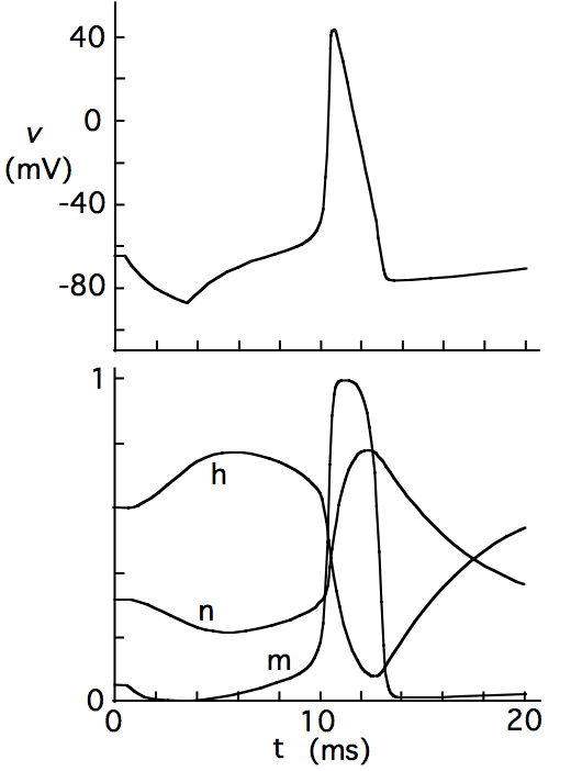
The internet has much information about how to view the eclipse safely. It is one of those topics where physics and medicine collide. In Chapter 14 of Intermediate Physics for Medicine and Biology, Russ Hobbie and I discuss the eye and vision. I won’t nag you about all the safety precautions. You can learn about them here.

How intense is the light reaching the retina when you stare at the sun? The intensity of sunlight at the earth’s surface is about 1 kW/m², or 1 mW/mm². The radius of the pupil is about 1 mm, and its area is approximately 3 mm². Therefore, about 3 mW impinges on the retina. To calculate the size of the image spot, treat the eye as a lens (Fig. 14.39a in IPMB). The earth-sun distance is 1.5 × 10⁸ km, the sun radius is 7 × 10⁵ km, and the pupil-retina distance is about 22 mm, implying that the radius of the sun’s image on the retina is (22 mm)(7 × 10⁵)/(1.5 × 10⁸) = 0.1 mm, for an area of about 0.03 mm². The intensity on the retina is thus 3 mW/.03 mm², or 100 mW/mm². This intensity will do damage.

Incidentally, if a 0.5 mW HeNe laser beam is directed into the eye and is focused to a spot with a radius of 0.04 mm, the intensity will be about the same as staring at the sun. Therefore, be as careful when playing with lasers as you are when viewing the eclipse. Both can be unsafe if you are careless.

Path of the total eclipse of the sun
in August 2017.

The light from the sun is about one million times as intense as the light from a full moon. The light from the sun’s corona, visible during a total eclipse, is about as bright as the full moon. So, when the eclipse is 99.99%, the sun is still one hundred times as bright as the moon. It is only when the eclipse is total that you can gaze at it safely. That's why I’m not going to Lawrence, Kansas—home of my alma mater the University of Kansas—for the event; there the eclipse is only 99.3% complete. (Vanderbilt, where I obtained my doctorate, is in the path of totality; my PhD advisor John Wikswo can watch it from his back yard.) We will drive for an hour (perhaps more, if traffic is snarled) to where the eclipse is total.

If you want to learn more, I suggest the “Resource Letter OSE-1: Observing Solar Eclipses,” written Jay Pasachoff and Andrew Fraknoi, and published by my favorite journal: The American Journal of Physics (Volume 85, Pages 485–494, July, 2017).

Enjoy!

Machines In Our Hearts

Machines in Our Hearts:
The Cardiac Pacemaker, the Implantable
Defibrillator, and American Health Care,
by Kirk Jeffrey.

In Chapter 7 of Intermediate Physics for Medicine and Biology, Russ Hobbie and I discuss pacemakers and defibrillators. When introducing this topic, we cite Kirk Jeffrey’s book Machines in Our Hearts: The Cardiac Pacemaker, the Implantable Defibrillator, and American Health Care. The book not only gives a great introduction to these medical devices, but also examines the medical device industry. In his introduction, Jeffrey writes

This book gives an account of the invention of the cardiac pacemaker and the subsequent development and transformation of this machine….The pacemaker was born in 1952 as an appliance the size of a breadbox that stood on a hospital cart and plugged into a wall socket. As it grew, it shrank. Within a few years, medical researchers and engineers had transformed it into a little device that was completely implanted within the patient’s body with one component actually threaded down a vein into the heart’s interior. Today we have a number of implanted machines, such as defibrillators and nerve stimulators, that manage some physiological function, but the pacemaker was the very first of these. Surgeons carried out the earliest implants in human beings between 1958 and 1960.

Pacemakers (or pacers) in the 1990s are no larger than wristwatches with one or two leads instead of a wristband. In the early days of implantable pacers, the devices were thicker and heavier than an old pocket watch; people in fact sometimes called them “heart tickers.” But a pacemaker today can do far more than send little ticks of electricity to the heart. Most pacers implanted in the 1990s coordinate the pumping action of the upper and lower chambers (the atria and ventricles) and change their rate depending on the patient’s activity level. Some can intervene to slow down a dangerously fast heartbeat. We live in “the age of the smart machine”; this phrase certainly applies to the newer pacers, for they include microprocessors and have become, in effect, computers…Once implanted, a pacemaker can be reprogrammed, its behavior completely reconfigured. In the near future, these tiny machines may be smart enough to diagnose the patient’s heart-rhythm problems and choose how to respond by themselves, without the doctor’s needing to intervene at all….

This book shifts its focus midway from the physicians and engineers who invented cardiac pacing and created a technological community to the manufacturing firms that have the greatest degree of control over the technology today. The manufacturers supplemented research physicians as the prime directors of technological change during the 1970s. The upshot is that when it comes to cardiac pacing and defibrillation, doctors are in effect working in alliance with large corporations in determining how best to treat patients.

Anyone interested in working in the medical device industry in general, and in designing new pacemakers and defibrillators in particular, should read Machines in Our Hearts. It is a case study of how physics can be applied to medicine and biology.

Suki is Going Deaf

Suki Roth, in front of a copy of
Intermediate Physics for
Medicine and Biology.

Suki is going deaf. She has not lost all her hearing yet, but when I call her in a normal voice she does not respond. She used to jump up when she heard me get the leash for a walk, but now I have to show it to her. Before she was scared of thunderstorms, but lately she snoozes through all but the loudest rumbles. In the past she got excited when the garage door opened, but nowadays she ignores it. Suki will be 15 years old this October, so such problems are expected. Still, I’m sad to see her sink into silence.

I think my hearing is getting worse too, but slowly. My dad uses a hearing aid, and I take after him. I find myself asking “what did you say?” more often than other people do. I decided to test myself using the website http://www.animations.physics.unsw.edu.au/jw/hearing.html. Below I plot my hearing (red dots) as a function of frequency, and compare it with the normal hearing response of a young adult (solid curve) shown in Figure 13.7 of Intermediate Physics for Medicine and Biology. I normalized the two curves so they are equal at 1 kHz.

My hearing response curve.

My hearing appears normal except for an odd deficit around 3000-4000 Hz. Also, I may be missing some high frequencies, but the loss is not dramatic.

I didn’t follow the website’s instructions exactly. I plotted the lowest intensity tone that I could just hear. I don’t trust this test, performed on myself using a website; it is very subjective and the loudness changes in large 3 dB steps. (In case you do not have IPMB handy, Eq. 13.34 indicates that a ten-fold change in intensity corresponds to a step of 10 in decibels.) I would be interested in hearing (get it?....) if you have a similar result using this website.

Age-related hearing loss is called presbycusis. Wikipedia says it is the second most common illness in the elderly, after arthritis. Normally we lose the high frequencies as we age, which has implications for how teenagers choose ringtones.

On the above video, I could hear the 8 kHz ringtone but not the 12 kHz or higher ones. Can you? I am not sure if it is me, my computer, or the video.

I may be losing some hearing, but probably not much. (Perhaps I just don’t pay attention when my wife talks to me.) Suki, however, is in worse shape. She is the world’s best pet, and I intend to give her extra treats to make up for her lack of hearing.

Do I Make Myself Clear?

Do I Make Myself Clear?
by Harold Evans.

I enjoy reading books about writing. Recently I read Do I Make Myself Clear? Why Writing Well Matters by Harold Evans. One of Evans’s pet peeves is “unnoticed redundancies, such as complete monopoly and awkward predicament, that do not add to the sense of the message.” He provides over 250 examples, with instructions to “strike out the words in italics.”

Of course, I became curious how Intermediate Physics for Medicine and Biology fared with these redundancies. So I hunted for them using the search box in my pdf version of IPMB. Most were absent, but a few appeared. I’m not sure they are always bad; you can decide for yourself. I enjoy doing this sort of thing, but is it fair to subject my dear readers to this analysis? I believe that writing well is critical for scientists; if pointing out some sloppy writing in IPMB can help others tighten their prose, the effort is worthwhile.

all of

Russ Hobbie and I occasionally include the unnecessary “of,” such as on page 59, “all of the external parameters,” which would sound tighter with no loss of meaning as “all the external parameters.”

a distance of

Evans puts the whole phrase in italics, which must mean he thinks it is unnecessary. Our text would probably be better by deleting “a distance of” from the homework problem on page 497: “Use the appropriate values for striated muscle to estimate the dose to the gonads if they are at a distance of 50 cm from the x-ray tube."

a number of examples

While Russ and I don’t use “a number of” with the word “examples,” we often write “a number of.” Sometimes we mean “several,” which I think is OK (although it sounds slightly pompous). My guess is that Evans is concerned primarily with cases when “a number of” could be deleted with no loss of meaning. I found a few examples in IPMB, such as on page 489, “irradiating the patient through a number of absorbers of different thickness spreads out the region of maximum dose” (and should it be “thicknesses”?), and especially page 514, “A number of more complicated situations are solved by Loevinger et al.”

a period of

I suspect that Evans is irritated by authors who write “a period of time,” which Russ and I never do. Sometimes we use “a period of” in the mathematical sense of the repeat time of a periodic function, such as on page 342: “If you are told that there is a signal in these data with a period of 4 s, you can group them together and average them.” No change is needed there. On the other hand, this text from page 39 is a borderline case: “figure 2.10 shows the survival of patients with congestive heart failure for a period of 9 years.” To me our prose sounds fine; I’m not sure what Evans would say.

appear to be

I admit, we occasionally have the unneeded “to be” after “appear,” such as on page 178 “does the charge distribution appear to be continuous or discrete?” and page 297 “do the results appear to be chaotic?” I write mainly be ear, and my ear isn’t bothered by “appear to be.” I am left wondering: “to be,” or not “to be,” that is the question.

as yet

On page 134 we write “There is evidence that some as yet unidentified toxin of medium molecular weight accumulates in the blood.” Yes, I concede the sentence would sound better if we delete the “as.”

close proximity

I agree with Evans that the “close” is bothersome. Russ and I never include a “close” with our “proximity,” except once on page 483 when we had no choice, it was inside a quote: “The bystander effect in radiobiology refers to the ‘induction of biological effects in cells that are not directly traversed by a charged particle, but are in close proximity to cells that are.’”

completely untrue

I think Evans’s point is that a statement can be either true or untrue, with no intermediate case, so completely is redundant. I’m not sure science is so black and white. Sometimes you can have an approximation that is very accurate, but technically untrue (Newtonian mechanics is almost true for speeds much less than the speed of light, but not completely true). Perhaps a better example is the cliché “completely pregnant.”

We have a lot of “completely”s in IPMB, most of which I am comfortable with. One questionable case appears on page 125: “if a solute is present to which the membrane is completely impermeable...” At first the completely sounds unneeded—a membrane is either permeable or it is not—but we had just introduced the hydraulic permeability, a parameter that can be very small without being zero. Saying “completely impermeable” is probably fine when we mean the limit as the hydraulic permeability goes to zero. I side with Evans that completely is unnecessary on page 88 “this differential form of the continuity equation is completely equivalent to the integral form,” and on page 279 “Jules Henri Poincaré realized around 1900 that systems described exactly by the completely deterministic equations of Newton’s laws could exhibit wild behavior.

depreciated in value

Although we don’t use “depreciated,” this wordy sentence from page 33 would be improved by deleting “in value”: “if the interest rate is 5% and if the interest is credited to the account once a year, the account increases in value by 5% of its present value each year.”

divide up

Russ and I sin only once, on page 144: “Divide up any closed surface into elements of surface area...”

end up

You tell me if this sentence form page 510 sounds better without the “up”; my ear can’t decide: “When a radiopharmaceutical is given to a patient for either diagnosis or therapy, the nuclei end up in different organs in varying amounts.”

have got

Sometimes Evans is like the Lorax: correct but annoying. I suppose this sentence from page 607 should not have the “gotten,” but the change seems so picky: “This is the same answer we would have gotten if h had been regarded as a constant.”

it is interesting to note that

We never use this exact phrase, but on page 248 “it is interesting to compare this to Eq. 9.38” would sound better as the command “compare this to Eq. 9.38.” I probably would not change page 11: “it is interesting to read what an orthopedic surgeon had to say about the use of a cane.”

past history

I hadn’t really thought about this redundancy until Evans pointed it out. He is right that “past history” is redundant, and I would change several such cases in IPMB, including page 57, “it is independent of the past history of the system and is specified by a few macroscopic parameters.”

Do I Make Myself Clear? is a fine book, although in my opinion it is not as good as Zinsser’s On Writing Well. Scientists are judged by their journal papers and grant proposals, both written documents. You need to write well, or your reputation will suffer. Eliminating minor redundancies is one way to make your writing clearer and more concise. Train your ear to listen for them.