The Eigenvalue Problem

An image of fiber tracts in the brain
using Diffusion Tensor Imaging.
From: Wikipedia.

In Intermediate Physics for Medicine and Biology, Russ Hobbie and I consider many mathematical topics. We analyze partial differential equations, Fourier transforms, vector calculus, probability, and special functions such as Bessel functions and the error function. One mathematical technique we never analyze is the central problem of linear algebra: the eigenvalue problem.

Calculating the eigenvalues and eigenvectors of a matrix has medical and biological applications. For example, in Chapter 18 of IPMB, Russ and I discuss diffusion tensor imaging. In this technique, magnetic resonance imaging is used to measure, in each voxel, the diffusion tensor, or matrix.

This matrix is symmetric, so D_xy = D_yx, etc. It contains information about how easily spins (primarily protons in water) diffuse throughout the tissue, and about the anisotropy of the diffusion: how the rate of diffusion changes with direction. White matter in the brain is made up of bundles of nerve axons, and spins can diffuse down the long axis of an axon much easier than in the direction perpendicular to it.

Suppose you measure the diffusion matrix to be

How do you get the fiber direction from this matrix? That is the eigenvalue and eigenvector problem. Stated mathematically, the fibers are in the direction of the eigenvector corresponding to the largest eigenvalue. In other words, you can determine a coordinate system in which the diffusion matrix becomes diagonal, and the direction corresponding to the largest of the diagonal elements of the matrix is the fiber direction.

The eigenvalue problem starts with the assumption that there are some vectors r = (x, y, z) that obey the equation Dr = Dr, where D in bold is the matrix (a tensor) and D in italics is one of the eigenvalues (a scalar). We can multiply the right side by the identity matrix (1’s along the diagonal, 0’s off the diagonal) and then move this term to the left side, and get the system of equations

One obvious solution is (x, y, z) = (0, 0, 0), the trivial solution. There is a beautiful theorem from linear algebra, which I will not prove, stating that there is a nontrivial solution for (x, y, z) if and only if the determinant of the matrix is zero

I am going to assume you know how to evaluate a determinant. From this determinant, you can obtain the equation

This is a cubic equation for D, which is in general difficult to solve. However, you can show that this equation is equivalent to

Therefore, the eigenvalues of this diffusion matrix are 4, 1, and 1 (1 is a repeated eigenvalue). The largest eigenvalue is D = 4.

To find the eigenvector associated with the eigenvalue D = 4, we solve

The solution is (1, 1, 1), which points in the direction of the fibers. If you do this calculation at every voxel, you generate a fiber map of the brain, leading to beautiful pictures such as you can see at the top of this post, and here or here.

Sometimes anisotropy can be a nuisance. Suppose you just want to determine the amount of diffusion in a tissue independent of direction. You can show (see Problem 49 of Chapter 18 in IPMB) that the trace of the diffusion matrix is independent of the coordinate system. The trace is the sum of the diagonal elements of the matrix. In our example, it is 2+2+2 = 6. In the coordinate system aligned with the fiber axis, the trace is just the sum of the eigenvalues, 4+1+1 = 6 (you have to count the repeated eigenvalue twice). The trace is the same.

Now you try. Here is a new homework problem for Section 13 in Chapter 18 of IPMB.

Problem 49 1/2. Suppose the diffusion tensor in one voxel is

a) Determine the fiber direction.

b) Show explicitly in this case that the trace is the same in the original matrix as in the matrix rotated so it is diagonal.

One word of warning. The examples in this blog post all happen to have simple integer eigenvalues. In general, that is not true and you need to use numerical methods to solve for the eigenvalues.

Have fun!

Darcy’s Law

Table 4.3 of Intermediate Physics for Medicine and Biology contains five transport equations. Each has the form “flux density equals a coefficient times the negative of a gradient of some quantity.” The table includes the flux of particles with the coefficient being the diffusion constant, the flux of heat with the coefficient being the thermal conductivity, the flux of momentum with the coefficient being the viscosity, and the flux of charge with the coefficient being the electrical conductivity. Are there other examples of transport equations important in biology and medicine? Yes. For instance, consider Darcy’s law.

Darcy’s law governs the flow of fluid through a porous medium. It is used to model the movement of groundwater through sedimentary rock, but it also describes the flow of water in tissue's extracellular space. Using a notation consistent with Table 4.3, we can write Darcy’s law as

j_v = - K dp/dx

where j_v is the flux density of fluid volume, p is the pressure, and K is the hydraulic conductivity. The units for j_v are m³ m^-2 s⁻¹, or m s⁻¹; therefore j_v corresponds to the speed of flow. Pressure has units of pascals, so dp/dx is expressed in Pa m⁻¹. Therefore, the units of hydraulic conductivity are m² Pa⁻¹ s⁻¹. Hydraulic conductivity is analogous to electrical conductivity or thermal conductivity; it specifies how well a material permits the transport of a quantity (flow of water) caused by some driving force (pressure gradient).

Russ Hobbie and I don’t discuss Darcy’s law in IPMB, but we come close. In Chapter 5 we analyze the flow of water across a membrane, and define the relationship

j_v = L_p Δp ,    (5.9)

where j_v again is the speed of flow, Δp is the pressure difference across the membrane, and L_p is the hydraulic permeability. If the membrane has a thickness Δx, then we can multiply and divide by Δx and obtain j_v = (L_p Δx) (Δp/Δx). The equation looks just like Darcy’s law (except for a minus sign), where the hydraulic conductivity is the hydraulic permeability times the membrane thickness:

K = L_p Δx.

I first encountered Darcy’s law when reading my friend Peter Basser’s paper about “Interstitial Volume, Pressure, and Flow During Infusion into the Brain” (Microvascular Research, 44:143–165, 1992). He derived a model of swelling in the brain that occurs during infusion of a drug. When Basser combined Darcy’s law with the equations of elasticity, he derived a diffusion equation for volume change of the tissue caused by accumulation of interstitial fluid (swelling), in which the diffusion constant is approximately the hydraulic conductivity times the bulk modulus.

Darcy’s law plays a key role in governing fluid flow in many tissues. A nice summary can be found in “Interstitial Flow and Its Effects in Solft Tissues” by Melody Swartz and Mark Fleury (Annual Review of Biomedical Engineering, 9:229–256, 2007). Below is the abstract to their review.

Interstitial flow plays important roles in the morphogenesis, function, and pathogenesis of tissues. To investigate these roles and exploit them for tissue engineering or to overcome barriers to drug delivery, a comprehensive consideration of the interstitial space and how it controls and affects such processes is critical. Here we attempt to review the many physical and mathematical correlations that describe fluid and mass transport in the tissue interstitium; the factors that control and affect them; and the importance of interstitial transport on cell biology, tissue morphogenesis, and tissue engineering. Finally, we end with some discussion of interstitial transport issues in drug delivery, cell mechanobiology, and cell homing toward draining lymphatics.

Strat-O-Matic Baseball

My Die-Hard Cub Fan Club
membership card.

Monday is opening day!

When I was young I was an avid baseball fan. I still enjoy the game, but now I haven’t time to follow it closely. My childhood team was the Chicago Cubs. I can still remember the lineup: shortstop Don Kessinger led off, second baseman Glenn Beckert hit next, left fielder Billy Williams batted third, and third baseman Ron Santo was cleanup. Ferguson Jenkins was the pitching ace, colorful Joe Pepitone—a former Yankee—arrived by trade to play first, Mr. Cub Ernie Banks was in the twilight of his career, and hot-tempered Leo Durochur was the manager. The Miracle Mets broke my heart in 1969, when the Cubs led their division into September only to collapse in the season's final weeks. The Cubs have not won the World Series since 1908, but I still love ’em. Maybe this year?

I wasn’t a good little league player; I struck out a lot, and I was assigned to play right field, where I could do the least damage with my glove. Yet, I had fun. One summer when I was in junior high, because of the timing of the age cutoffs and my birthday, I was nearly the oldest player in my age group. That was my best summer, when I approached mediocrity. I enjoyed the sport so much that I volunteered to manage the high school team. For those not familiar with baseball, being the manager in high school is very different than managing a professional team. In high school, the manager washes the uniforms, keeps track of the equipment, collects player statistics, and—my favorite job—draws the foul lines on the field before each game.

Strat-O-Matic Baseball.

When growing up in Morrison, Illinois, my friend Ted Paul owned the game Strat-O-Matic Baseball. It was played with dice and player cards, allowing you to recreate baseball games from your armchair. Unfortunately, Strat-O-Matic Baseball was expensive. We were not poor, but the price was out of the range my parents spent on birthday or Christmas presents. Necessity is the mother of invention, so I reverse engineered the game, making my own cards and rules that mimicked Strat-O-Matic’s in some ways but in other ways were my own creation.

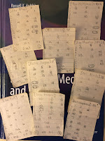
Homemade Strat-O-Matic baseball cards
from the Oakland A’s, the dominant team
of that era (circa 1973).

In order to make my version of Strat-O-Matic Baseball, I had to learn the basics of probability. I didn’t need advanced concepts, and you can find all the necessary probability theory in Chapter 3 of Intermediate Physics for Medicine and Biology. Two ideas are key. First, the probability that one or the other of two mutually exclusive events happens is found by adding their individual probabilities. For instance, the probability of rolling either a one, two, or three on a single die is equal to the probability of rolling a one plus the probability of rolling a two plus the probability of rolling a three. Second, the probability that two independent events both happen is found by multiplying their individual probabilities. For example, the probability of throwing a one on the first die and a three on the second is equal to the probability of throwing a one times the probability of throwing a three. This concept underlies the joint probability distribution described in Appendix M of IPMB. These two rules, plus some counting, is all the math required to recreate Strat-O-Matic baseball. I also needed a source of baseball statistics, supplied by Street and Smith’s Baseball Yearbook, published each year around Valentine's Day and well within the family gift budget. In retrospect, making my own version of Strat-O-Matic Baseball was not difficult, but for a twelve-year-old kid I think I did a pretty good job.

Let me explain briefly how Strat-O-Matic Baseball works. The game was based on batters’ cards and pitchers’ cards. First you roll one die, and if you get a 1, 2, or 3 you use the batter’s card; a 4, 5, or 6 means you use the pitcher's card. Then you roll two dice which determine the outcome of the at-bat: out, walk, single, double, triple, or home run. The trick is to match the player’s statistics to the probability of a particular throw of the dice. The pitchers’ cards were hardest to create, because Street and Smith didn’t tabulate batting averages given up by pitchers, so I had to invent an algorithm based on wins, earned run average, and strikeouts. I remember spending many hours playing my homemade Strat-O-Matic baseball. In some ways it was pathetic: a child playing alone in his room with just his dice and cards. But in other ways it was romantic: thrilling late night ballgames with all the drama and excitement of sports, but performed just for me.

Even now, when I teach probability I focus on those key concepts I used when creating my version of Strat-O-Matic Baseball. Sometimes you learn more when you play than when you work.

Basic Physics of Nuclear Medicine

I’m cheap and I’m proud of it; I love free stuff. Intermediate Physics for Medicine and Biology isn’t free. Russ Hobbie and I appreciate our readers’ willingness to spend their money to purchase our book. Thank you! But what if you want more? What if—heaven forbid—you find our book is not totally clear, complete, or comprehensive? In IPMB we cite many references at the end of each chapter, so you have many sources of additional information. But often these sources cost money or may be difficult to obtain. Is there anywhere you can go online for free to augment IPMB?

A screenshot of the wikibook
Basic Physics of Nuclear Medicine.

One option is the wikibook Basic Physics of Nuclear Medicine. This book covers much of the same material as in the last half of IPMB. It analyzes in depth nuclear medicine (our Chapter 17), but it also covers the interaction of radiation with tissue (our Chapter 15), Fourier methods and tomography (our Chapters 11 and 12), detectors and x-ray imaging systems (our Chapter 16), ultrasound (our Chapter 13), and even a little magnetic resonance imaging (our Chapter 18).

Some of my favorite parts of the wikibook are not covered in IPMB:

• An analysis of using dual-energy radiography to remove the bones from an x-ray image.
• A chapter on computers in nuclear medicine.
• A discussion of the Picture Archiving and Communication System (PACS) and image processing.
• An overview of three dimensional visualization techniques.

What are the advantages of IPMB? For one thing, IPMB has a large collection of homework problems, more extensive than in Basic Physics of Nuclear Medicine. Also, I think our book has a better focus on using mathematical modeling to illustrate medical and biological physics concepts. Moreover, the entire first half of IPMB—about biomechanics, biothermodynamics, diffusion, bioelectricity, biomagnetism, and feedback—is absent from Basic Physics of Nuclear Medicine. Finally, and most importantly, Basic Physics of Nuclear Medicine doesn’t have a blog with weekly updates.

If you are looking for a free, easily accessible online textbook to use as a supplement (please, not a replacement!) for Intermediate Physics for Medicine and Biology, consider Basic Physics of Nuclear Medicine. It’s worth every penny.

Phineas Gage: Neuroscience’s Most Famous Patient

When Russ Hobbie and I discuss transcranial magnetic stimulation in Intermediate Physics for Medicine and Biology, we write that “because TMS is noninvasive and nearly painless, it can be used to study learning and plasticity (changes in brain organization over time).” When I worked with Mark Hallett and Leo Cohen at the National Institutes of Health, they were using TMS to study plasticity in patients who had undergone amputations or spinal cord injuries.

Phineas Gage.

How much can the brain reorganize and rehabilitate after an injury? We gain insight into this question by examining the amazing case of Phineas Gage. Recently, science writer Sam Kean published the article “Phineas Gage, Neuroscience’s Most Famous Patient” in the online magazine Slate. Let me quote Kean’s opening lines.

On Sept. 13, 1848, at around 4:30 p.m., the time of day when the mind might start wandering, a railroad foreman named Phineas Gage filled a drill hole with gunpowder and turned his head to check on his men. It was the last normal moment of his life….

The Rutland and Burlington Railroad had hired Gage’s crew that fall to clear away some tough black rock near Cavendish, Vermont, and it considered Gage the best foreman around. Among other tasks, a foreman sprinkled gunpowder into blasting holes, and then tamped the powder down, gently, with an iron rod. This completed, an assistant poured in sand or clay, which got tamped down hard to confine the bang to a tiny space. Gage had specially commissioned his tamping iron from a blacksmith. Sleek like a javelin, it weighed 13¼ pounds and stretched 3 feet 7 inches long. (Gage stood 5-foot-6.) At its widest, the rod had a diameter of 1¼ inches, although the last foot—the part Gage held near his head when tamping—tapered to a point.

Gage’s crew members were loading some busted rock onto a cart, and they apparently distracted him. Accounts differ about what happened after Gage turned his head. One says Gage tried to tamp the gunpowder down with his head still turned, and scraped his iron against the side of the hole, creating a spark. Another says Gage’s assistant (perhaps also distracted) failed to pour the sand in, and when Gage turned back, he smashed the rod down hard, thinking he was packing inert material. Regardless, a spark shot out somewhere in the dark cavity, igniting the gunpowder, and the tamping iron rocketed upward.

The iron entered Gage’s head point-first, striking below the left cheekbone. It destroyed an upper molar, passed behind his left eye, and tore into the underbelly of his brain’s left frontal lobe. It then plowed through the top of his skull, exiting near the midline, just behind where his hairline started. After parabola-ing upward—one report claimed it whistled as it flew—the rod landed 25 yards away and stuck upright in the dirt, mumblety-peg-style. Witnesses described it as streaked with red and greasy to the touch, from fatty brain tissue.

Gage survived after his rod destroyed much of his frontal lobe. He eventually recovered much neural function, but his personality changed; Gage “was no longer Gage”. At least, so goes the traditional story as told in many neuroscience textbooks. Kean argues that these personality changes were not as dramatic as claimed, and were temporary. Years after the accident, Gage enjoyed fairly good health and lived a nearly normal life. His brain recovered. Kean writes

Modern neuroscientific knowledge makes the idea of Gage’s recovery all the more plausible. Neuroscientists once believed that brain lesions caused permanent deficits: Once lost, a faculty never returned. More and more, though, they recognize that the adult brain can relearn lost skills. This ability to change, called brain plasticity, remains somewhat mysterious, and it happens achingly slowly. But the bottom line is that the brain can recover lost functions in certain circumstances.

If transcranial magnetic stimulation had been developed in the first half of the nineteenth century (and why not? Faraday discovered electromagnetic induction 17 years before Gage’s accident), perhaps neuroscientists would have had the tool they needed to monitor and map Gage’s brain during his recovery. Magnetic stimulation—a classic application of physics to medicine—has taught us much about how the brain can change and heal. This knowledge might have implications for how we treat all sorts of brain injuries, from concussion to stroke to dementia to rods shot through our head. As Kean concludes, “If even Phineas Gage bounced back—that’s a powerful message of hope.”

Mass Attenuation Coefficient and Areal Density

I don’t like the mass attenuation coefficient; it bugs me and it has weird units. Yet researchers studying the attenuation of x-rays in materials usually quote the mass attenuation coefficient rather than the linear attenuation coefficient in their publications.

As x-rays pass through a material, they fall off exponentially as exp(−μL), where L is the distance (m) and μ is the linear attenuation coefficient (m⁻¹). But often researchers multiply and divide by the density ρ, so the exponential becomes exp(−(μ/ρ)(ρL)), where μ/ρ is the mass attenuation coefficient (m²/kg) and ρL is the areal density (kg/m²).

In Chapter 15 of Intermediate Physics of Medicine and Biology, Russ Hobbie and I explain some of the advantages of using μ/ρ.

The mass attenuation coefficient has the advantage of being independent of the density of the target material, which is particularly useful if the target is a gas. It has an additional advantage if Compton scattering is the dominant interaction. If σ_tot = Zσ_C, then μ_atten/ρ = Zσ_CN_A/A [Z is the atomic number, A the mass number, N_A is Avogadro’s number, and σ_C is the Compton cross section]. Since Z/A is nearly 1/2 for all elements except hydrogen, this quantity changes very little throughout the periodic table. This constancy is not true for the photoelectric effect or pair production. Figure 15.10 plots the mass attenuation coefficient vs energy for three substances spanning the periodic table. It is nearly independent of Z around 1 MeV where Compton scattering is dominant. The K and L absorption edges can be seen for lead; for the lighter elements they are below 10 keV. Figure 15.11 shows the contributions to μ_atten/ρ for air from the photoelectric effect, incoherent scattering, and pair production. Tables of mass attenuation coefficients are provided by the National Institute of Standards and Technology (NIST) at http://www.nist.gov/pml/data/xcom/index.cfm.

Let me offer an example where it makes sense to consider the mass attenuation coefficient.

Imagine you have a large box of area S. You measure a mass M of the fluid pentane and poor it into the box. Then you place a source of x-rays under the box, directed upwards. You measure the intensity of the radiation incident on the underside of the box to be I_o, and then move your detector to above the box and measure the intensity of radiation that passes through the pentane to be I. Finally, use your ruler to measure the thickness of the pentane layer, L.

You now have enough data to determine both the linear attenuation coefficient and the mass attenuation coefficient of pentane. For the linear attenuation coefficient, use the relationship I = I_o exp(−μL) and solve for μ = ln(I_o/I)/L. You can also calculate the density ρ = M/(SL). If you want the mass attenuation coefficient, you can now easily determine it: S ln(I_o/I)/M. You can also calculate the areal density: M/S.

Next you perform the same experiment on neopentane. You use the same box with area S and measure out the same mass M of fluid. You find that I_o/I is unchanged, but L is about 6% larger. You conclude the linear attenuation coefficient and the density both decrease by 6%, but the mass attenuation coefficient and the areal density are unchanged.

Why is I_o/I the same for both fluids? Pentane and neopentane are isomers. They have exactly the same chemical formula, C₅H₁₂, but they have different structures. Pentane is an unbranched hydrocarbon and neopentane has a central carbon bonded to four other carbon atoms. Because the mass M of both substances is the same, the number of the atoms is the same in each case. The x-ray attenuation only depends on the number of atoms and the type of atoms, but not how those atoms are arranged (the density). This is one advantage of the mass attenuation coefficient: it depends only on the atoms and not their arrangement.

You can calculate the mass attenuation coefficient and the areal density without knowing L. If for some reason L were difficult to measure, you could still determine the mass attenuation coefficient even if you could not calculate the linear attenuation coefficient.

In a gas, the number of molecules is fixed but the density depends on the pressure and temperature. The mass attenuation coefficient does not change with the pressure and temperature. Again, it just depends on the atoms and not their distribution.

Water has a density of 1 g/cm³. If you express the mass attenuation coefficient in cm²/g and the linear attenuation coefficient in cm, then the mass attenuation coefficient and the linear attenuation coefficient have the same numerical value. Most tissue has a density close to that of water, so this trick works well for tissue too.

Given these advantages, have I started liking the mass attenuation coefficient? No, I still think it’s weird. But I can tolerate it a little better now.

Welcome Home Scott Kelly

Scott Kelly, when he returned to earth
after a year on the space station.

This week astronaut Scott Kelly returned to Earth after nearly a year on the International Space Station. One goal of his mission was to determine how astronauts would function during long trips in space. I suspect we will learn a lot from Kelly about life in a weightless environment. But one of the biggest risks during a mission to Mars would be radiation exposure, and we may not learn much about that from trips to the space station.

In space, the major source of radiation is cosmic rays, consisting mostly of high energy (GeV) protons. Most of these particles are absorbed by our atmosphere and never reach Earth, or are deflected by Earth’s magnetic field. The space station orbits above the atmosphere but within range of the geomagnetic field, so Kelly was partially shielded from cosmic rays. He probably experienced a dose of about 150 mSv. This is much larger than the annual background dose on the surface of the earth. According to Chapter 16 of Intermediate Physics for Medicine and Biology, we all are exposed to about 3 mSv per year.

Scott and Mark Kelly.

Is 150 mSv in one year dangerous? This dose is below the threshold for acute radiation sickness. It would, however, increase your chances of developing cancer. A rule of thumb is that the excess relative risk of cancer is about 5% per Sv. This does not mean Kelly has a 0.75% chance of getting cancer (5%/Sv times 0.15 Sv). Instead, it means that Scott Kelly has a 0.75% higher chance of getting cancer than his brother Mark Kelly, who remained on Earth. This is a significant increase in risk, but may be acceptable if your goal in life is to be an astronaut. The Kelly twins are both 52 years old, and the excess relative risk goes down with age, so the extra risk of Scott Kelly contracting cancer is probably less than 0.5%.

NASA’s goal is to send astronauts to Mars. Such a mission would require venturing beyond the range of Earth’s geomagnetic field, increasing the exposure to cosmic rays. Data obtained by the Mars rover Curiosity indicate that a one-year interplanetary trip would result in an exposure of 660 mSv. This would be four times Kelly's exposure in the space station. 660 mSv would be unlikely to cause serious acute radiation sickness, but would increase the cancer risk. NASA would have to either shield the astronauts from cosmic rays (not easy given their high energy) or accept the increased risk. I’m guessing they will accept the risk.

Top 10 Isotopes

Everyone loves “top ten” lists. So, I have prepared a list of the top ten isotopes mentioned in Intermediate Physics for Medicine and Biology. These isotopes range from light to heavy, from abundant to rare, and from mundane to exotic. I have no statistics to back up my choices; they are just my own view about which isotopes play a key role in biology and medicine. Feel free to sound off in the comments about your favorite isotope that I missed. Let’s count them down to number one.

10. ¹H (hydrogen-1). This simplest of all isotopes has a nucleus that consists of only a single proton. Almost all magnetic resonance imaging is based on imaging ¹H (see Chapter 18 of IPMB about MRI). Its importance arises from its large abundance and its nuclear dipole moment.
9. ²²²Rn (radon-222). While radon doesn’t have a large role in nuclear medicine, it is responsible for a large fraction of our annual background radiation dose (see Chapter 16 about the medical uses of x-rays). ²²²Rn is created in a decay chain starting with the long-lived isotope ²³⁸U. Because radon is a noble gas, it can diffuse out of uranium-containing rocks and enter the air, where we breathe it in, exposing our lungs to its alpha particle decay.
8. ¹³¹I (iodine-131). ¹³¹I is used in the treatment of thyroid cancer. Iodine is selectively taken up by the thyroid, where it undergoes beta decay, providing a significant dose to the surrounding tissue. A tenth of its radiation arises from gamma decay, so we can use the isotope for both imaging and therapy (see Chapter 17 about nuclear medicine).
7. ¹⁹²Ir (iridium-192). This gamma emitter is often used in stents placed in blocked arteries. It is also an important source for brachytherapy (Chapter 17), when a radioactive isotope is implanted in a tumor.
6. ¹²⁹Xe (xenon-129). This isotope is used in magnetic resonance images of the lung. Although the isotope is not abundant, its polarization can be increased dramatically using a technique called hyperpolarization (Chapter 18).
5. ¹⁰B (boron-10). This isotope of boron plays the central role in boron neutron capture therapy (Chapter 16). in which boron-containing drugs accumulate in a tumor. When irradiated by neutrons, the boron decays into an alpha particle (⁴He) and ⁷Li, which both have high energy and are highly ionizing.
4. ⁶⁰Co (cobalt-60). For many years cobalt-60 was used as a source of radiation during cancer therapy (Chapter 16). The gamma knife uses ⁶⁰Co sources to produce its 1.25 MeV radiation. The isotope is used less nowadays, replaced by linear accelerators.
3. ¹²⁵I (iodine-125). Iodine is the only element with two isotopes in this list. Unlike ¹³¹I, which emits penetrating beta and gamma rays, ¹²⁵I deposits much of its energy in short-range Auger electrons (see Chapter 15 on the interaction of x-rays with matter). They deliver a large, concentrated dose when ¹²⁵I is used for radioimmunotherapy.
2. ¹⁸F (florine-18). A classic positron emitter, ¹⁸F is widely used in positron emission tomography (Chapter 17). Often it is attached to the sugar molecule as ¹⁸F-fluorodeoxyglucose, which is taken up and is then trapped inside cells, providing a PET marker for high metabolic activity.
1. ^99mTc (technitium-99m). The king of all nuclear medicine isotopes, ^99mTc is used in diverse imaging applications (Chapter 17). It emits a 141-keV gamma ray that is ideal for most detectors. The isotope is often bound to other molecules to produce specific radiopharmaceuticals, such as ^99mTc-sestamibi or ^99mTc-tetrofosmin. If you are only familiar with one isotope used in nuclear medicine, let it be ^99mTc.