Showing posts sorted by date for query 150. Sort by relevance Show all posts

Friday, September 9, 2022

An Immense World

“Earth teems with sights and textures, sounds and vibrations, smells and tastes, electric and magnetic fields. But every animal can only tap into a small fraction of reality’s fullness. Each is enclosed within its own unique sensory bubble, perceiving but a tiny sliver of our immense world.”
An Immense World, by Ed Yong, superimposed on Intermediate Physics for Medicine and Biology.
An Immense World,
by Ed Yong.
Those three sentences sum up Ed Yong’s new book An Immense World: How Animal Senses Reveal the Hidden Realms Around Us. Yong is a science writer for The Atlantic who won a Pulitzer Prize for his reporting about the COVID-19 pandemic. I’ve mentioned Yong in this blog before when quoting advice from his chapter in the book Science Blogging: “you have to have something worth writing about, and you have to write it well.” In An Immense World, Yong does both.

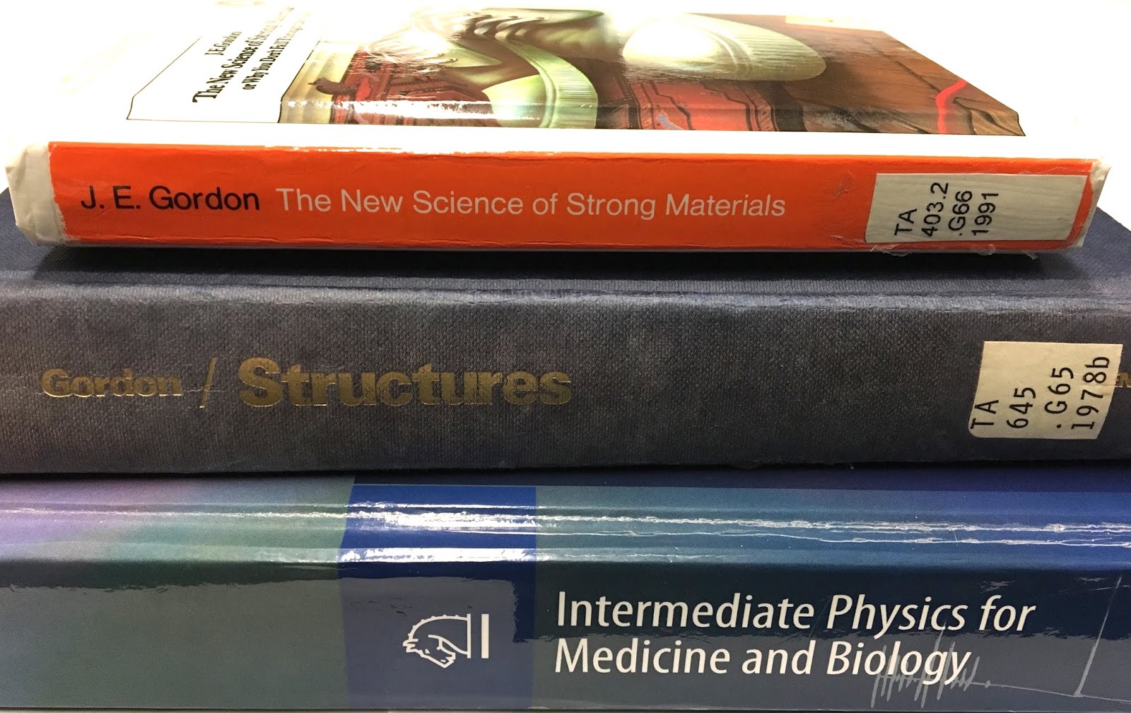
An Immense World sometimes overlaps with Intermediate Physics for Medicine and Biology. For example, both books discuss vision. Yong points out the human eye has better visual acuity than most other animals. He writes “we assume that if we can see it, they [other animals] can, and that if it’s eye-catching to us, it’s grabbing their attention… That’s not the case.” Throughout his book, Yong returns to this idea of how sensory perception differs among animals, and how misleading it can be for us to interpret animal perceptions from our own point of view.

Like IPMB, An Immense World examines color vision. Yong speculates about what a bee would think of the color red, if bees could think like humans.
Imagine what a bee might say. They are trichromats, with opsins that are most sensitive to green, blue, and ultraviolet. If bees were scientists, they might marvel at the color we know as red, which they cannot see and which they might call “ultrayellow” [I would have thought “infrayellow”]. They might assert at first that other creatures can’t see ultrayellow, and then later wonder why so many do. They might ask if it is special. They might photograph roses through ultrayellow cameras and rhapsodize about how different they look. They might wonder whether the large bipedal animals that see this color exchange secret messages through their flushed cheeks. They might eventually realize that it is just another color, special mainly in its absence from their vision.
Both An Immense World and IPMB also analyze hearing. Yong says
Human hearing typically bottoms out at around 20 Hz. Below those frequencies, sounds are known as infrasound, and they’re mostly inaudible to us unless they’re very loud. Infrasounds can travel over incredibly long distances, especially in water. Knowing that fin whales also produce infrasound, [scientist Roger] Payne calculated, to his shock, that their calls could conceivably travel for 13,000 miles. No ocean is that wide.…

Like infrasound, the term ultrasound… refers to sound waves with frequencies higher than 20 kHz, which marks the upper limit of the average human ear. It seems special—ultra, even—because we can’t hear it. But the vast majority of mammals actually hear very well into that range, and it’s likely that the ancestors of our group did, too. Even our closest relatives, chimpanzees, can hear close to 30 kHz. A dog can hear 45 kHz; a cat, 85 kHz; a mouse, 100 kHz; and a bottlenose dolphin, 150 kHz. For all of these creatures, ultrasound is just sound.
In IPMB, Russ Hobbie and I introduce the decibel scale for measuring sound intensity, or how loud a sound is. Yong uses this concept when discussing bats.
The sonar call of the big brown bat can leave its mouth at 138 decibels—roughly as loud as a siren or jet engine. Even the so-called whispering bats, which are meant to be quiet, will emit 110-decibel shrieks, comparable to chainsaws and leaf blowers. These are among the loudest sounds of any land animal, and it’s a huge mercy that they’re too high-pitched for us to hear.

Yong examines senses that Russ and I never consider, such as smell, taste, surface vibrations, contact, and flow. He wonders about the relative value of nociception [a reflex action to avoid a noxious stimulus] and the sensation of pain [a subjective feeling created by the brain].

The evolutionary benefit of nociception is abundantly clear. It’s an alarm system that allows animals to detect things that might harm or kill them, and take steps to protect themselves. But the origin of pain, on top of that, is less obvious. What is the adaptive value of suffering?

On the continuum ranging from life’s unity to diversity, Yong excels at celebrating the diverse, while Russ and I focus on how physics reveals unifying principles. I’m sometimes frustrated that Yong doesn’t delve into the physics of these topics more, but I am in awe of how he highlights so many strange and wonderful animals. There’s a saying that “nothing in biology makes sense except in light of evolution.” That’s true for An Immense World, which is a survey of how the evolution of sensory perception shapes they way animals interact, mate, hunt their prey, and avoid their predators.

Two chapters of An Immense World I found especially interesting were about sensing electric and magnetic fields. When discussing the black ghost knifefish’s ability to sense electric fields, Yong writes

Just as sighted people create images of the world from patterns of light shining onto their retinas, an electric fish creates electric images of its surroundings from patterns of voltage dancing across its skin. Conductors shine brightly upon it. Insulators cast electric shadows.
Then he notes that
Fish use electric fields not just to sense their environment but also to communicate. They court mates, claim territory, and settle fights with electric signals in the same way other animals might use colors or songs.
Even bees can detect electric fields. For instance, the 100 V/m electric field that exists at the earth’s surface can be sensed by bees.
Although flowers are negatively charged, they grow into the positively charged air. Their very presence greatly strengthens the electric fields around them, and this effect is especially pronounced at points and edges, like leaf tips, petal rims, stigmas, and anthers. Based on its shape and size, every flower is surrounded by its own distinctive electric field. As [scientist Daniel] Robert pondered these fields, “suddenly the question came: Do bees know about this?” he recalls. “And the answer was yes.”
The chapter on sensing magnetic fields is different from the others, because we don’t yet know how animals sense these fields.
Magnetoreception research has been polluted by fierce rivalries and confusing errors, and the sense itself is famously difficult both to study and to comprehend. There are open questions about all the senses, but at least with vision, smell, or even electroreception, researchers know roughly how they work and which sense organs are involved. Neither is true for magnetoreception. It remains the sense that we know least about, even though its existence was confirmed decades ago.

Yong lists three possible mechanisms for magnetoreception: 1) magnetite, 2) electromagnetic induction, and 3) magnetic effects on radical pairs. Russ and I discuss the first two in IPMB. I get the impression that the third is Yong’s favorite, but I remain skeptical. In my book Are Electromagnetic Fields Making Me Ill? I say that “they jury is still out” on the radical pair hypothesis.

If you want to read a beautifully written book that explores how much of the physics in Intermediate Physics for Medicine and Biology can be used by species throughout the animal kingdom to sense their environment, I recommend An Immense World. You’ll love it.

 Umwelt: The hidden sensory world of animals. By Ed Yong.

https://www.youtube.com/watch?v=Pzsjw-i6PNc


 Ed Yong on An Immense World

https://www.youtube.com/watch?v=bQS0Ioch05E

Friday, July 9, 2021

The Bragg Peak

In Chapter 16 of Intermediate Physics for Medicine and Biology, Russ Hobbie and I discuss the Bragg peak.
Protons are also used to treat tumors (Khan 2010, Ch. 26; Goitein 2008). Their advantage is the increase of stopping power at low energies. It is possible to make them come to rest in the tissue to be destroyed, with an enhanced dose relative to intervening tissue and almost no dose distally (“downstream”) as shown by the Bragg peak in Fig.16.47.
Energy loss versus depth for a 150 MeV proton beam in water, with and without straggling (fluctuations in the range). The Bragg peak enhances the energy deposition at the end of the proton range. Adapted from Fig. 16.47 in Intermediate Physics for Medicine and Biology.

William Henry Bragg, discoverer of the Bragg peak.
William Henry Bragg
Sir William Henry Bragg
(1862 – 1942) was an English scientist who shared the 1915 Nobel Prize in Physics with his son Lawrence Bragg for their analysis of crystal structure using X-rays. In 2004, Andrew Brown and Herman Suit published an article commemorating “The Centenary of the Discovery of the Bragg Peak” (Radiotherapy and Oncology, Volume 73, Pages 265-268).
In December 1904, William Henry Bragg, Professor of Mathematics and Physics at the University of Adelaide and his assistant Richard Kleeman published in the Philosophical Magazine (London) novel observations on radioactivity. Their paper “On the ionization of curves of radium,” gave measurements of the ionization produced in air by alpha particles, at varying distances from a very thin source of radium salt. The recorded ionization curves “brought to light a fact, which we believe to have been hitherto unobserved. It is, that the alpha particle is a more efficient ionizer towards the extreme end of its course.” This was promptly followed by further results in the Philosophical Magazine in 1905. Their finding was contrary to the accepted wisdom of the day, viz. that the ionizations produced by alpha particles decrease exponentially with range. From theoretical considerations, they concluded that an alpha particle possesses a definite range in air, determined by its initial energy and produces increasing ionization density near the end of its range due to its diminishing speed.
Although Bragg discovered the Bragg peak for alpha particles, the same behavior is found for other heavy charged particles such as protons. It is the key concept underlying the development of proton therapy. Brown and Suit conclude
The first patient treatment by charged particle therapy occurred within a decade of Wilson’s paper [the first use of protons in therapy, published in 1946]. Since then, the radiation oncology community has been evaluating various particle beams for clinical use. By December 2004, a century after Bragg’s original publication, the approximate number of patients treated by proton–neon beams is 47,000 (Personal communication, Janet Sisterson, Editor, Particles) [over 170,000 today]. There have been several clear clinical gains. None of these would have been possible, were it not for the demonstration that radically different depth dose curves were feasible.

Friday, June 4, 2021

The Bidomain Model of Cardiac Tissue: Predictions and Experimental Verification

“The Bidomain Model of Cardiac Tissue: Predictions and Experimental Verification” superimopsed on Intermediate Physics for Medicine and Biology.
“The Bidomain Model of Cardiac Tissue:
Predictions and Experimental Verification”

In the early 1990s, I was asked to write a chapter for a book titled Neural Engineering. My chapter had nothing to do with nerves, but instead was about cardiac tissue analyzed with the bidomain model. (You can learn more about the bidomain model in Chapter 7 of Intermediate Physics for Medicine and Biology.) 

“The Bidomain Model of Cardiac Tissue: Predictions and Experimental Verification” was submitted to the editors in January, 1993. Alas, the book was never published. However, I still have a copy of the chapter, and you can download it here. Now—after nearly thirty years—it’s obsolete, but provides a glimpse into the pressing issues of that time.

I was a impudent young buck back in those days. Three times in the chapter I recast the arguments of other scientists (my competitors) as syllogisms. Then, I asserted that their premise was false, so their conclusion was invalid (I'm sure this endeared me to them). All three syllogisms dealt with whether or not cardiac tissue could be treated as a continuous tissue, as opposed to a discrete collection of cells.

The Spach Experiment

The first example had to do with the claim by Madison Spach that the rate of rise of the cardiac action potential, and time constant of the action potential foot, varied with direction.

Continuous cable theory predicts that the time course of the action potential does not depend on differences in axial resistance with direction.

The rate of rise of the cardiac wave front is observed experimentally to depend on the direction of propagation.

Therefore, cardiac tissue does not behave like a continuous tissue.
I then argued that their first premise is incorrect. In one-dimensional cable theory, the time course of the action potential doesn’t depend on axial resistance, as Spach claimed. But in a three-dimensional slab of tissue superfused by a bath, the time course of the action potential depends on the direction of propagation. Therefore, I contended, their conclusion didn’t hold; their experiment did not prove that cardiac tissue isn’t continuous. To this day the issue is unresolved.

Defibrillation

A second example considered the question of defibrillation. When a large shock is applied to the heart, can its response be predicted using a continuous model, or are discrete effects essential for describing the behavior?
An applied current depolarizes or hyperpolarizes the membrane only in a small region near the ends of a continuous fiber.

For successful defibrillation, a large fraction of the heart must be influenced by the stimulus.

Therefore, defibrillation cannot be explained by a continuous model.
I argued that the problem is again with the first premise, which is true for tissue having “equal anisotropy ratios” (the same ratio of conductivity parallel and perpendicular to the fibers, in both the intracellular and extracellular spaces), but is not true for “unequal anisotropy ratios.” (Homework Problem 50 in Chapter 7 of IPMB examines unequal anisotropy ratios in more detail). If the premise is false, the conclusion is not proven. This issue is not definitively resolved even today, although the sophisticated simulations of realistically shaped hearts with their curving fiber geometry, performed by Natalia Trayanova and others, suggest that I was right.

Reentry Induction

The final example deals with the induction of reentry by successive stimulation through a point electrode. As usual, I condensed the existing dogma to a syllogism.
In a continuous tissue, the anisotropy can be removed by a coordinate transformation, so reentry caused by successive stimulation through a single point electrode cannot occur, since there is no mechanism to break the directional symmetry.

Reentry has been produced experimentally by successive stimulation through a single point electrode.

Therefore, cardiac tissue is not continuous.

Once again, that pesky first premise is the problem. In tissue with equal anisotropy ratios you can remove anisotropy by a coordinate transformation, so reentry is impossible. However, if the tissue has unequal anisotropy ratios the symmetry is broken, and reentry is possible. Therefore, you can’t conclude that the observed induction of reentry by successive stimulation through a point electrode implies the tissue is discrete.


I always liked this book chapter, in part because of the syllogisms, in part because of its emphasis on predictions and experiments, but mainly because it provides a devastating counterargument to claims that cardiac tissue acts discretely. Although it was never published, I did send preprints around to some of my friends, and the chapter took on a life of its own. This unpublished manuscript has been cited 13 times!

Trayanova N, Pilkington T (1992) “The use of spectral methods in bidomain studies,” Critical Reviews in Biomedical Engineering, Volume 20, Pages 255–277.

Winfree AT (1993) “How does ventricular tachycardia turn into fibrillation?” In: Borgreffe M, Breithardt G, Shenasa M (eds), Cardiac Mapping, Mt. Kisco NY, Futura, Chapter 41, Pages 655–680.

Henriquez CS (1993) “Simulating the electrical behavior of cardiac tissue using thebidomain model,” Critical Reviews of Biomedical Engineering, Volume 21, Pages 1–77.

Wikswo JP (1994) “The complexities of cardiac cables: Virtual electrode effects,” Biophysical Journal, Volume 66, Pages 551–553.

Winfree AT (1994) “Puzzles about excitable media and sudden death,” Lecture Notes in Biomathematics, Volume 100, Pages 139–150.

Roth BJ (1994) “Mechanisms for electrical stimulation of excitable tissue,” Critical Reviews in Biomedical Engineering, Volume 22, Pages 253–305.

Roth BJ (1995) “A mathematical model of make and break electrical stimulation ofcardiac tissue by a unipolar anode or cathode,” IEEE Transactions on Biomedical Engineering, Volume 42, Pages 1174–1184.

Wikswo JP Jr, Lin S-F, Abbas RA (1995) “Virtual electrodes in cardiac tissue: A common mechanism for anodal and cathodal stimulation,” Biophysical Journal, Volume 69, Pages 2195–2210.

Roth BJ, Wikswo JP Jr (1996) “The effect of externally applied electrical fields on myocardial tissue,” Proceedings of the IEEE, Volume 84, Pages 379–391.

Goode PV, Nagle HT (1996) “On-line control of propagating cardiac wavefronts,” The 18th Annual International Conference of the IEEE Engineering in Medicine and Biology Society, Amsterdam.

Winfree AT (1997) “Rotors, fibrillation, and dimensionality,” In: Holden AV, Panfilov AV (eds): Computational Biology of the Heart, Chichester, Wiley, Pages 101–135.

Winfree AT (1997) “Heart muscle as a reaction-diffusion medium: The roles of electric potential diffusion, activation front curvature, and anisotropy,” International Journal of Bifurcation and Chaos, Volume 7, Pages 487–526.

Winfree AT (1998) “A spatial scale factor for electrophysiological models of myocardium,” Progress in Biophysics and Molecular Biology, Volume 69, Pages 185–203.
I’ll end with the closing paragraph of the chapter.
The bidomain model ignores the discrete nature of cardiac cells, representing the tissue as a continuum instead. Experimental evidence is often cited to support the hypothesis that the discrete nature of the cells plays a key role in cardiac electrophysiology. In each case, the bidomain model offers an alternative explanation for the phenomena. It seems wise at this point to reconsider the evidence that indicates the significance of discrete effects in healthy cardiac tissue. The continuous bidomain model explains the data, recorded by Spach and his colleagues, showing different rates of rise during propagation parallel and perpendicular to the fibers, anodal stimulation, arrhythmia development by successive stimulation from a point source, and possibly defibrillation. Of course, these alternative explanations do not imply that discrete effects are not responsible for these phenomena, but only that two possible mechanisms exist rather than one. Experiments must be found that differentiate unambiguously between alternative models. In addition, discrete junctional resistance must be incorporated into the bidomain model. Only when such experiments are performed and the models are further developed will we be able to say with any certainty that cardiac tissue can be described as a continuum.

Friday, December 11, 2020

Selig Hecht (1892-1947)

A photo of Selig Hecht
Selig Hecht,
History of the Marine Biological Laboratory,
http://hpsrepository.asu.edu/handle/10776/3269.
In Chapter 14 of Intermediate Physics for Medicine and Biology, Russ Hobbie and I analyze the “classic experiment on scotopic vision” by Hecht, Shlaer, and Pirenne. George Wald wrote an obituary about Selig Hecht in 1948 (Journal of General Physiology, Volume 32, Pages 1–16). He writes that Hecht was
Intensely interested in the relation of light quanta (photons) to vision. Reexamining earlier measurements of the minimum threshold for human rod vision, he and his colleagues confirmed that vision requires only fifty to 150 photons. When all allowances had been made for surface reflections, the absorption of light by ocular tissues, and the absorption by rhodopsin (which alone is an effective stimulant), it emerged that the minimum visual sensation corresponds to the absorption in the rods of, at most, five to fourteen photons. An entirely independent statistical analysis suggested that an absolute threshold involves about five to seven photons. Both procedures, then, confirmed the estimation of the minimum visual stimulus at five to fourteen photons. Since the test field in which these measurements were performed contained about 500 rods, it was difficult to escape the conclusion that one rod is stimulated by a single photon.
Wald also describes the coauthor on the study, Shlaer.
Among Hecht’s first students was Simon Shlaer, who became Hecht’s assistant in his first year at Columbia and continued as his associate for twenty years thereafter. A man infinitely patient with things and impatient with people, Shlaer gave Hecht his entire devotion. He was a master of instrumentation, and though he also had a keen grasp of theory, he devoted himself by choice to the development of new technical devices. Hecht and Shlaer built a succession of precise instruments for visual measurement, among them an adaptometer and an anomaloscope that have since gone into general use. The entire laboratory came to rely on Shlaer’s ingenuity and skill. “I am like a man who has lost his right arm,” remarked Hecht on leaving Columbia—and Shlaer—in 1947, “and his right leg.”

In his Columbia laboratory, Hecht instituted investigations of human dark adaptation, brightness discrimination, visual acuity, the visual response to flickered light, the mechanism of the visual threshold, and normal and anomalous color vision. His lab also made important contributions regarding the biochemistry of visual pigments, the relation of night blindness to vitamin A deficiency in humans, the spectral sensitivities of man and other animals, and the light reactions of plants—phototropism, photosynthesis, and chlorophyll formation.
Hecht and Shlaer both contributed to the war effort during the Second World War.
Throughout the late years of World War II, Hecht devoted his energies and the resources of his laboratory to military problems. He and Shlaer developed a special adaptometer for night-vision testing that was adopted as standard equipment by several Allied military services. Hecht also directed a number of visual projects for the Army and Navy and was consultant and advisor on many others. He was a member of the National Research Council Committee on Visual Problems and of the executive board of the Army-Navy Office of Scientific Research and Development Vision Committee.

Explaining the Atom, by Selig Hecht, superimposed on Intermediate Physics for Medicine and Biology.
Explaining the Atom,
by Selig Hecht.
Hecht straddled the fields of physics and physiology, and was comfortable with both math and medicine. He entered college studying mathematics. After World War II ended, he wrote the book Explaining the Atom, which Wald described as “a lay approach to atomic theory and its recent developments that the New York Times (in a September 20, 1947, editorial) called ‘by far the best so far written for the multitude.’”

An obituary in Nature by Maurice Henri Pirenne concludes

The death of Prof. Selig Hecht in New York on September 18, 1947, at the age of fifty-five, deprives the physiology of vision of one of its most outstanding workers. Hecht was born in Austria and was brought to the United States as a child. He studied and worked in the United States, in England, Germany and Italy. After a broad biological training, he devoted his life to the study of the mechanisms of vision, considered as a branch of general physiology. He became professor of biophysics at Columbia University and made his laboratory an international centre of visual research.

Friday, July 24, 2020

Tests for Human Perception of 60 Hz Moderate Strength Magnetic Fields

The first page of “Tests for Human Perception of 60 Hz Moderate Strength Magnetic Fields,” by Tucker and Schmitt (IEEE Trans. Biomed. Eng. 25:509-518, 1978), superimposed on Intermediate Physics for Medicine and Biology.
The first page of “Tests for Human Perception
of 60 Hz Moderate Strength Magnetic Fields,”
by Tucker and Schmitt (IEEE Trans. Biomed. Eng.
25:509-518, 1978).
In Chapter 9 of Intermediate Physics for Medicine and Biology, Russ Hobbie and I discuss possible effects of weak external electric and magnetic fields on the body. In a footnote, we write
Foster (1996) reviewed many of the laboratory studies and described cases where subtle cues meant the observers were not making truly “blind” observations. Though not directly relevant to the issue under discussion here, a classic study by Tucker and Schmitt (1978) at the University of Minnesota is worth noting. They were seeking to detect possible human perception of 60-Hz magnetic fields. There appeared to be an effect. For 5 years they kept providing better and better isolation of the subject from subtle auditory clues. With their final isolation chamber, none of the 200 subjects could reliably perceive whether the field was on or off. Had they been less thorough and persistent, they would have reported a positive effect that does not exist.
In this blog, I like to revisit articles that we cite in IPMB.
Robert Tucker and Otto Schmitt (1978) “Tests for Human Perception of 60 Hz Moderate Strength Magnetic Fields.” IEEE Transactions on Biomedical Engineering, Volume 25, Pages 509-518.
The abstract of their paper states
After preliminary experiments that pointed out the extreme cleverness with which perceptive individuals unintentionally used subtle auxiliary clues to develop impressive records of apparent magnetic field detection, we developed a heavy, tightly sealed subject chamber to provide extreme isolation against such false detection. A large number of individuals were tested in this isolation system with computer randomized sequences of 150 trials to determine whether they could detect when they were, and when they were not, in a moderate (7.5-15 gauss rms) alternating magnetic field, or could learn to detect such fields by biofeedback training. In a total of over 30,000 trials on more than 200 persons, no significantly perceptive individuals were found, and the group performance was compatible, at the 0.5 probability level, with the hypothesis that no real perception occurred.
The Tucker-Schmitt study illustrates how observing small effects can be a challenge. Their lesson is valuable, because many weak-field experiments are subject to systematic errors that provide an illusion of a positive result. Near the start of their article, Tucker and Schmitt write
We quickly learned that some individuals are incredibly skillful at sensing auxiliary non-magnetic clues, such as coil hum associated with field, so that some “super perceivers” were found who seemed to sense the fields with a statistical probability as much as 10–30 against happening by chance. A vigorous campaign had then to be launched technically to prevent the subject from sensing “false” clues while leaving him completely free to exert any real magnetic perceptiveness he might have.
Few authors are as forthright as Tucker and Schmitt when recounting early, unsuccessful experiments. Yet, their tale shows how experimental scientists work.
Early experiments, in which an operator visible to the test subject controlled manually, according to a random number table, whether a field was to be applied or not, alerted us to the necessity for careful isolation of the test subject from unintentional clues from which he could consciously, or subconsciously, deduce the state of coil excitation. No poker face is good enough to hide, statistically, knowledge of a true answer, and even such feeble clues as changes in building light, hums, vibrations and relay clatter are converted into low but significant statistical biases.
IPMB doesn’t teach experimental methods, but all scientists must understand the difference between systematic and random errors. Uncertainty from random errors is suppressed by taking additional data, but eliminating systematic errors may require you to redesign your experiment.
In a first round of efforts to prevent utilization of such clues, the control was moved to a remote room and soon given over to a small computer. A “fake” air-core coil system, remotely located but matched in current drain and phase angle to the real large coil system was introduced as a load in the no-field cases. An acoustically padded cabinet was introduced to house the experimental subject, to isolate him from sound and vibration. Efforts were also made to silence the coils by clamping them every few centimeters with plastic ties and by supporting them on air pocket packing material. We tried using masking sound and vibrations, but soon realized that this might also mask real perception of magnetic fields.
Designing experiments is fun; you get to build stuff in a machine shop! I imagine Tucker and Schmitt didn’t expect they would have this much fun. Their initial efforts being insufficient, they constructed an elaborate cabinet to perform their experiments in.
This cabinet was fabricated with four layers of 2 in plywood, full contact epoxy glued and surface coated into a monolithic structure with interleaved corners and fillet corner reinforcement to make a very rigid heavy structure weighing, in total, about 300 kg. The structure was made without ferrous metal fastening and only a few slender brass screws were used. The door was of similar epoxyed 4-ply construction but faced with a thin bonded melamine plastic sheet. The door was hung on two multi-tongue bakelite hinges with thin brass pins. The door seals against a thin, closed-cell foam-rubber gasket, and is pressure sealed with over a metric ton of force by pumping a mild vacuum inside the chamber of means of a remote acoustically silenced hose-connected large vacuum-cleaner blower. The subject received fresh air through a small acoustic filter inlet leak that also assures sufficient air flow to cool the blower. The chosen “cabin altitude” at about 2500 ft above ambient presented no serious health hazard and was fail-safe protected.
An experimental scientist must be persistent. I remember learning that lesson as a graduate student when I tried for weeks to measure the magnetic field of a single nerve axon. I scrutinized every part of the experiment and fixed every problem I could find, but I still couldn’t measure an action current. Finally, I realized the coaxial cable connecting the nerve to the stimulator was defective. It was a rookie mistake, but I was tenacious and ultimately figured it out. Tucker and Schmitt personify tenacity.
As still more isolation seemed necessary to guarantee practically complete exclusion of auxiliary acoustic and mechanical clues, an extreme effort was made to improve, even further, the already good isolation. The cabinet was now hung by aircraft “Bungee” shock cord running through the ceiling to roof timbers. The cabinet was prevented from swinging as a pendulum by four small non-load-bearing lightly inflated automotive type inner tubes placed between the floor and the cabinet base. Coils already compliantly mounted to isolate intercoil force vibration were very firmly reclamped to discourage intracoil “buzzing.” The cabinet was draped inside with sound absorbing material and the chair for the subject shock-mounted with respect to the cabinet floor. The final experiments, in which minimal perception was found, were done with this system.
Once Tucker and Schmitt heroically eliminated even the most subtle cues about the presence of a magnetic field, subjects could no longer detect whether or not a magnetic field was present. People can’t perceive 60-Hz, 0.0015-T magnetic fields.

Russ and I relegate this tale to a footnote, but it’s an important lesson when analyzing the effects of weak electric and magnetic fields. Small systematic errors abound in these experiments, both when studying humans and when recording from cells in a dish. Experimentalists must ruthlessly design controls that can compensate for or eliminate confounding effects. The better the experimentalist, the more doggedly they root out systematic errors. One reason the literature on the biological effects of weak fields is so mixed may be that few experimentalists take the time to eradicate all sources of error.

Tucker and Schmitt’s experiment is a lesson for us all.

Friday, December 28, 2018

The Pitfalls of Using Handbooks and Formulae

A photo of three books: (left) Structures: Or Why Things Don't Fall Down, (center) Intermediate Physics for Medicine and Biology, and (right) The New Science of Strong Materials: Or Why You Don’t Fall Through the Floor.
Structures: Or Why Things Don't Fall Down, by J. E. Gordon.
Last week I discussed James Gordon’s book Structures: Or Why Things Don’t Fall Down. The book contains several appendices. The first appendix is ostensibly about using handbooks and formulas to make structural calculations.
Over the last 150 years the theoretical elasticians have analysed the stresses and deflections of structures of almost every conceivable shape when subjected to all sorts and conditions of loads…Fortunately a great deal of this information has been reduced to a set of standard cases or examples the answers to which can be expressed in the form of quite simple formulae.
Then, to my surprise, Gordon changes tack and warns about pitfalls when using these formulas. His counsel, however, applies to all calculations, not just mechanical ones. In fact, his advice is invaluable for any young scientist or engineer. Below, I quote parts of this appendix. Read carefully, and whenever you encounter a word specific to mechanics substitute a general one, or one related to your own field.
[Formulae] must be used with caution.
A photo of Appendix 1 from Structures: Or Why Things Don't Fall Down, superimposed on the cover of Intermediate Physics for Medicine and Biology.
Appendix 1 of Structures.
  1. Make sure that you really understand what the formula is about.
  2. Make sure that it really does apply to your particular case.
  3. Remember, remember, remember, that these formulae take no account of stress concentrations or other special local conditions.
After this, plug the appropriate loads and dimensions into the formula—making sure that the units are consistent and that the noughts are right. [I’m not sure what “noughts” are, but I think the Englishman Gordon is saying to make sure the decimal point is in the right place.] Then do a little elementary arithmetic and out will drop a figure representing a stress or a deflection.

Now look at this figure with a nasty suspicious eye and think if it looks and feels right. In any case you had better check your arithmetic; are you sure that you haven’t dropped a two?...

If the structure you propose to have made is an important one, the next thing to do, and a very right and proper thing, is to worry about it like blazes. When I was concerned with the introduction of plastic components into aircraft I used to lie awake night after night worrying about them, and I attribute the fact that none of these components ever gave trouble almost entirely to the beneficent effects of worry. It is confidence that causes accidents and worry which prevents them. So go over your sums not once or twice but again and again and again.
Appendix 1 in J. E. Gordon's book Structures: Or Why Things Don't Fall Down has an important lesson for students studying from Intermediate Physics for Medicine and Biology.
Structures: Or Why Things Don't Fall Down.
This is the attitude I try to instill in my students when teaching from Intermediate Physics for Medicine and Biology. I implore them to think before they calculate, and then think again to judge if their answer makes sense. Students sometimes submit an answer to a homework problem (almost always given to five or six significant figures) that is absurd because they didn't look at their answer with a “nasty suspicious eye.” I insist they "remember, remember, remember" the assumptions and limitations of a mathematical model and its resulting formulas. Maybe Gordon goes a little overboard with his “night after night” of lost sleep, but at least he cares enough about his calculation to wonder “again and again and again” if it is correct. A little worry is indeed a “right and proper thing.”

Who would of expected such wisdom tucked away in an appendix about handbooks and formulae?

Friday, May 25, 2018

The Constituents of Blood

Intermediate Physics for Medicine and Biology: The Constituents of BloodI’m a big supporter of blood donation. This week I gave another pint to the Red Cross, which brings my total to 8 gallons. As I lay there with a needle stuck in my arm, I began to wonder “what’s in this blood they’re squeezing out of me?”

Table 3.1 in Intermediate Physics for Medicine and Biology lists some constituents of blood. I reproduce the table below, with revisions.

Constituent Density in mg/cm3 Number in 1 μm3
Water 1000 33,000,000,000
Sodium 3 83,000,000
Glucose 1 3,300,000
Cholesterol 2 3,100,000
Hemoglobin 150 1,400,000
Albumin 45 390,000

This version of the table highlights several points. Water molecules outnumber all others by a factor of four hundred. Sodium ions are sixty times more common than hemoglobin molecules, but the mass density of hemoglobin is over fifty times that of sodium. In other words, if judged by number of molecules (and therefore the osmotic effect) sodium is most important, but if judged by mass or volume fraction, hemoglobin dominates. Glucose and cholesterol are intermediate cases. Albumin has a surprisingly small number of molecules, given that I thought it was one of the main contributors to osmotic pressure. It is a big molecule, however, so by mass it contributes nearly a third as much as hemoglobin.

Are other molecules in blood important? You can find a comprehensive list of blood constituents beautifully illustrated here. When judged by number, sodium is the most important small ion, but the chloride ion contributes nearly as much. Carbon dioxide and bicarbonate are also significant, and potassium has about the same number of molecules as glucose. If you drive drunk, you may have twice as many ethyl alcohol molecules as potassium ions (if the number of ethanol molecules reaches the level of sodium or chloride ions, you die). Urea has a similar number of molecules as hemoglobin.

Judged by mass, you get an entirely different picture. Large protein molecules dominate. Hemoglobin is by far the largest contributor to blood by mass (after water, of course), followed by albumin and another group of proteins called globulins. Next are glycoproteins such as the clotting factor fibrinogen and iron-binding transferrin.

Many trace constituents hardly affect the osmotic pressure or density of blood, but are excellent biomarkers for diagnosing diseases.

If you’re starting to think that blood is awfully crowded, you’re right. The picture below is by David Goodsell. No scale bar is included, but each candy-apple-red hemoglobin molecule in the lower left has a diameter of about 6 nm. The water, ions, and other small molecules such as glucose are not shown; if they had been they would produce a fine granular appearance (water has diameter of about 0.3 nm) filling in the spaces between the larger macromolecules.

Blood. Illustration by David S. Goodsell, the Scripps Research Institute.
Blood. Serum is in the upper right and a red blood cell is in the lower left. In the serum, the Y-shaped molecules are antibodies (an immunoglobulin), the long thin light-red molecules are fibrinogen (a glycoprotein), and the numerous potato-like yellow proteins are albumin. The red blood cell is filled with red hemoglobin molecules. The cell membrane is in purple. The illustration is by David S. Goodsell of the Scripps Research Institute.

In another eight weeks I will get free juice and cookies be eligible to give blood again. It doesn’t hurt (much) or take (too) long. If you want to donate, contact the American Red Cross. Give the gift of life.

Friday, March 30, 2018

The Radiation Dose from Radon: A Back-of-the-Envelope Estimation

Intermediate Physics for Medicine and Biology: The Radiation Dose from Radon I like Fermi problems: those back-of-the-envelope order-of-magnitude estimates that don’t aim for accuracy, but highlight underlying principles. I also enjoy devising new homework exercises for the readers of this blog. Finally, I am fascinated by radon, that radioactive gas that contributes so much to the natural background radiation. Ergo, I decided to write a new homework problem about estimating the radiation dose from breathing radon.

What a mistake. The behavior of radon is complex, and the literature is complicated and confusing. Part of me regrets starting down this path. But rather than give up, I plan to forge ahead and to drag you—dear reader—along with me.
Section 17.12
Problem 57 1/2. Estimate the annual effective dose (in Sv yr-1) if the air contains a trace of radon. Use the data in Fig. 17.27, and assume the concentration of radon corresponds to an activity of 150 Bq m-3, which is the action level at which the Environmental Protection Agency suggests you start to take precautions. Make reasonable guesses for any parameters your need.
Here is my solution (stop reading now if you first want to solve the problem yourself). In order to be accessible to a wide audience, I avoid jargon and unfamiliar units.
One bequerel is a decay per second, and a cubic meter is 1000 liters, so we start with 0.15 decays per second per liter. The volume of air in your lungs is about 6 liters, implying that approximately one atom of radon decays in your lungs every second.

Radon decays by emitting an alpha particle. You don’t, however, get just one. Radon-222 (the most common isotope of radon) alpha-decays to polonium-218, which alpha-decays to lead-214, which beta-decays twice to polonium-214, which alpha-decays to lead-210 (see Fig 17.27 in Intermediate Physics for Medicine and Biology). The half-life of lead-210 is so long (22 years) that we can treat it as stable. Each decay of radon therefore results in three alpha particles. An alpha particle is ejected with an energy of about 6 MeV. Therefore, roughly 18 MeV is deposited into your lungs each second. If we convert to SI units (1 MeV = 1.6 × 10⁻¹³ joule), we get about 3 × 10-12 joules per second.

Absorbed dose is expressed in grays, and one gray is a joule per kilogram. The mass of the lungs is about 1 kilogram. So, the dose rate for the lungs is 3 × 10-12 grays per second. To find the annual dose, multiply this dose rate by one year, or 3.2 × 10⁷ seconds. The result is about 10-4 gray, or a tenth of a milligray per year.

If you want the equivalent dose in sieverts, multiply the absorbed dose in grays by 20, which is the radiation weighting factor for alpha particles. To get the effective dose, multiply by the tissue weighting factor for the lungs, 0.12. The final result is 0.24 mSv per year.
This all seems nice and logical, except the result is a factor of ten too low! It is probably even worse than that, because my initial radon concentration was higher than average and in Table 16.6 of IPMB Russ Hobbie and I report a value of 2.28 mSv for the average annual effective dose. My calculation here is an estimate, so I don’t expect the answer to be exact. But when I saw such a low value I was worried and started to read some of the literature about radon dose calculations. Here is what I learned:
  1. The distribution of radon progeny (such as 214Po) is complicated. These short-lived isotopes are charged and behave differently than an unreactive noble gas like radon. They stick to particles in the air. Your dose depends on how dusty the air is.
  2. How these particles interact with our lungs is even more difficult to understand. Some large particles are filtered out by the upper respiratory track
  3. The range of a 6-MeV alpha particle is only about 50 microns, so some of the energy is deposited harmlessly into the gooey mucus layer lining the airways (see https://www.ncbi.nlm.nih.gov/books/NBK234233). Ironically, if you get bronchitis your mucus layer thickens, protecting you from radon-induced lung cancer.  
  4. The progeny and their dust particles stick to the bronchi walls like flies to flypaper, increasing their concentration.
  5. Filtering out dust and secreting a mucus layer reduces the dose to the lungs, while attaching the progeny to the airway lining increases it. My impression from the literature is that the flypaper effect dominants, and explains why my estimate is so low.
  6. The uranium-238 decay chain shown in Fig. 17.27 is the source of radon-222, but other isotopes arise from other decay chains. The thorium-232 decay chain leads to radon-220, called thoron, which also contributes to the dose.
  7. I am not confident about my value for the mass. The lungs are a bloody organ; about half of their mass is blood. I don’t know whether or not the blood is included in the reported 1 kg mass. The radon literature is oddly silent about the lung mass, and I don’t know how these authors calculate the dose without it. 
  8. I ignored the energy released when progeny beta-decay, which would cause a significant error if my aim was to calculate the absorbed dose in grays. But if I want the effective dose in sieverts I should be alright, because the radiation weighting factor for electrons is 1 compared to 20 for alpha particles. 
  9. The radon literature is difficult to follow in part because of strange units, such as picocuries per liter and working level months (see https://www.ncbi.nlm.nih.gov/books/NBK234224).
  10. Radon can get into the water as well as the air. If you drink the water, your stomach gets a dose. With a half-life of days, the radon in this elixir has time to enter your blood and irradiate your entire body.
  11. Does the dose from radon lead to lung cancer? That depends on the accuracy of the linear no-threshold model. If there is a threshold, then such a small dose may not represent a risk.
  12. If you want to learn more about radon, read NCRP Report 160, ICRP Publication 103, or BEIR VI. Of course, you should start by reading Section 17.12 in IPMB.
What do I take away from this estimation exercise? First, radon dosimetry is complicated. Second, biology problems are messy, and while order-of-magnitude estimates are still valuable, your results need large error bars.

Friday, November 10, 2017

Facebook

The logo for the Intermediate Physics for Medicine and Biology Facebook page.
The Intermediate Physics for Medicine and Biology Facebook Group has now reached 150 members.

Yes, IPMB has a Facebook group. I use it to circulate blog posts every Friday morning, but I occasionally share other posts of interest to readers of IPMB. The group photo is my Ideal Bookshelf picture highlighting books about physics applied to medicine and biology.

Group members include my family (including my dog Suki Roth, who has her own Facebook Page) and former students. But members I don’t know come from countries all over the world, including:
In particular, many members are from India and Pakistan.

I am amazed and delighted to have members from all over the world. I don’t know if universities teach classes based on IPMB in all these places, or if people just stumble upon the group.

The IPMB Facebook group welcomes everyone interested in physics applied to medicine and biology. I am delighted to have you. And for those who are not yet members, just go to Facebook, search for “Intermediate Physics for Medicine and Biology,” and click “Join Group.” Let’s push for 200 members!

Friday, December 30, 2016

The Story of the World in 100 Species

The Story of the World  in 100 Species,  by Christopher Lloyd, superimposed on Intermediate Physics for Medicine and BIology.
The Story of the World
in 100 Species,
by Christopher Lloyd.
I recently finished reading The Story of the World in 100 Species. The author Christopher Lloyd writes in the introduction
This book is a jargon-free attempt to explain the phenomenon we call life on Earth. It traces the history of life from the dawn of evolution to the present day through the lens of one hundred living things that have changed the world. Unlike Charles Darwin’s theory published more than 150 years ago, it is not chiefly concerned with the “origin of species,” but with the influence and impacts that living things have had on the path of evolution, on each other and on our mutual environment, planet Earth.
Of course, I began to wonder how many of the top hundred species Russ Hobbie and I mention in Intermediate Physics for Medicine and Biology. Lloyd lists the species in order of impact. The number 1 species is the earthworm. As Darwin understood, you would have little agriculture without worms churning the soil. The highest ranking species that was mentioned in IPMB is number 2, algae, which produces much of the oxygen in our atmosphere. According to Lloyd, algae might provide the food (ick!) and fuel we need in the future.

Number 6 is ourselves: humans. Although the species name Homo sapiens never appears in IPMB, several chapters—those dealing with medicine—discuss us. Number 8 yeast (specifically, S. cerevisiae) is not in IPMB, although it is mentioned previously in this blog. Number 15 is the fruit fly Drosophila melanogaster, which made the list primarily because it is an important model species for research. IPMB mentions D. melanogaster when discussing ion channels.

Cows are number 17; a homework problem in IPMB contains the phrase “consider a spherical cow.” The flea is number 18, and is influential primarily for spreading diseases such as the Black Death. In IPMB, we analyze how fleas survive high accelerations. Wheat reaches number 19 and is one of several grains on the list. In Chapter 11, Russ and I write: “Examples of pairs of variables that may be correlated are wheat price and rainfall, ….” I guess that wheat is in IPMB, although the appearance is fairly trivial. Like yeast, number 20 C. elegans, a type of roundworm, is never mentioned in IPMB but does appear previously in this blog because it is such a useful model. I am not sure if number 21, the oak tree, is in IPMB. My electronic pdf of the book has my email address, roth@oakland.edu, as a watermark at the bottom of every page. Oak is not in the appendix, and I am pretty sure Russ and I never mention it, but I haven’t the stamina to search the entire pdf, clicking on each page. I will assume oak does not appear.

Number 24, grass, gets a passing mention: in a homework problem about predator-prey models, we write that “rabbits eat grass…foxes eat only rabbits.” When I searched the book for number 25 ant, I found constant, quantum, implant, elephant, radiant, etc. I gave up after examining just a few pages. Let’s say no for ant. Number 28 rabbit is in that predator-prey problem. Number 32 rat is in my favorite J. B. S. Haldane quote “You can drop a mouse down a thousand-yard mine shaft; and arriving at the bottom, it gets a slight shock and walks away. A rat is killed, and man is broken, a horse splashes.” Number 33 bee is in the sentence “Bees, pigeons, and fish contain magnetic particles,” and number 38 shark is in the sentence “It is possible that the Lorentz force law allows marine sharks, skates, and rays to orient in a magnetic field.” My favorite species, number 42 dog, appears many times. I found number 44 elephant when searching for ant. I am not sure about number 46 cat (complicated, scattering, indicate, cathode, … you search the dadgum pdf!). It doesn’t matter; I am a dog person and don’t care for cats.

Number 53 apple; IPMB suggests watching Russ Hobbie in a video about the program MacDose at the website https://itunes.apple.com/us/itunes-u/photon-interactions-simulation/id448438300?mt=10. No way am I counting that; you gotta draw the line somewhere. Number 58 horse; “…horse splashes…”. Number 59 sperm whale; we mention whales several times, but don’t specify the species—I’m counting it. Number 61 chicken appears in one of my favorite homework problems: “compare the mass and metabolic requirements…of 180 people…with 12,600 chickens…” Number 65 red fox; see predator-prey problem. Number 67 tobacco; IPMB mentions it several times. Number 71 tea; I doubt it but am not sure (instead, steady, steam, ….). Number 77 HIV; see Fig. 1.2. Number 85 coffee; see footnote 7, page 258.

Altogether, IPMB includes twenty of the hundred species (algea, human, fruit fly, cow, flea, wheat, grass, rabbit, rat, bee, shark, dog, elephant, horse, whale, chicken, fox, tobacco, HIV, coffee), which is not as many as I expected. We will have to put more into the 6th edition (top candidates: number 9 influenza, number 10 penicillium, number 14 mosquito, number 26 sheep, number 35 maize aka corn).

Were any important species missing from Lloyd’s list? He includes some well-known model organisms (S. cerevisiae, D. melanogaster, C. elegans) but inexplicably leaves out the bacterium E. coli (Fig. 1.1 in IPMB). Also, I am a bioelectricity guy, so I would include Hodgkin and Huxley’s squid with its giant axon. Otherwise, I think Lloyd’s list is pretty complete.

If you want to get a unique perspective on human history, learn some biology, and better appreciate evolution, I recommend The Story of the World in 100 Species.

Friday, March 4, 2016

Welcome Home Scott Kelly

A photograph of Scott Kelly, when he returned to earth after a year on the space station.
Scott Kelly, when he returned to earth
after a year on the space station.
This week astronaut Scott Kelly returned to Earth after nearly a year on the International Space Station. One goal of his mission was to determine how astronauts would function during long trips in space. I suspect we will learn a lot from Kelly about life in a weightless environment. But one of the biggest risks during a mission to Mars would be radiation exposure, and we may not learn much about that from trips to the space station.

In space, the major source of radiation is cosmic rays, consisting mostly of high energy (GeV) protons. Most of these particles are absorbed by our atmosphere and never reach Earth, or are deflected by Earth’s magnetic field. The space station orbits above the atmosphere but within range of the geomagnetic field, so Kelly was partially shielded from cosmic rays. He probably experienced a dose of about 150 mSv. This is much larger than the annual background dose on the surface of the earth. According to Chapter 16 of Intermediate Physics for Medicine and Biology, we all are exposed to about 3 mSv per year.

A photograph of Scott and Mark Kelly.
Scott and Mark Kelly.
Is 150 mSv in one year dangerous? This dose is below the threshold for acute radiation sickness. It would, however, increase your chances of developing cancer. A rule of thumb is that the excess relative risk of cancer is about 5% per Sv. This does not mean Kelly has a 0.75% chance of getting cancer (5%/Sv times 0.15 Sv). Instead, it means that Scott Kelly has a 0.75% higher chance of getting cancer than his brother Mark Kelly, who remained on Earth. This is a significant increase in risk, but may be acceptable if your goal in life is to be an astronaut. The Kelly twins are both 52 years old, and the excess relative risk goes down with age, so the extra risk of Scott Kelly contracting cancer is probably less than 0.5%.

NASA’s goal is to send astronauts to Mars. Such a mission would require venturing beyond the range of Earth’s geomagnetic field, increasing the exposure to cosmic rays. Data obtained by the Mars rover Curiosity indicate that a one-year interplanetary trip would result in an exposure of 660 mSv. This would be four times Kelly's exposure in the space station. 660 mSv would be unlikely to cause serious acute radiation sickness, but would increase the cancer risk. NASA would have to either shield the astronauts from cosmic rays (not easy given their high energy) or accept the increased risk. I’m guessing they will accept the risk.

Friday, November 9, 2012

The Hydrogen Spectrum

One of the greatest accomplishments of atomic physics is Neils Bohr’s model for the structure of the hydrogen atom, and his prediction of the hydrogen spectrum. While Bohr gets the credit for deriving the formula for the wavelengths, λ, of light emitted by hydrogen—one of the early triumphs of quantum mechanics—it was first discovered empirically from the spectroscopic analysis of Johannes Rydberg. In the 4th edition of Intermediate Physics for Medicine and Biology, Russ Hobbie and I introduce Rydberg’s formula in Homework Problem 4 of Chapter 14.
Problem 4 (a) Starting with Eq. 14.7, derive a formula for the hydrogen atom spectrum in the form

The hydrogen spectrum.

where n and m are integers. R is called the Rydberg constant. Find an expression for R in terms of fundamental constants. 
(b) Verify that the wavelengths of the spectral lines a-d at the top of Fig. 14.3 are consistent with the energy transitions shown at the bottom of the figure.
Our Fig. 14.3 is in black and white. It is often useful to see the visible hydrogen spectrum (just four lines, b-e in Fig 14.3) in color, so you can appreciate better the position of the emission lines in the spectrum.

(Figure from http://chemed.chem.purdue.edu/genchem/topicreview/bp/ch6/graphics/hydrogen.gif).

The hydrogen lines in the visible part of the spectrum are often referred to as the Balmer series, in honor of physicist Johann Balmer who discovered this part of the spectrum before Rydberg. Additional Balmer series lines exist in the near ultraviolet part of the spectrum (the thick band of lines just to the left of line e at the top of Fig. 14.3). All the Balmer series lines can be reproduced using the equation in Problem 4 with n = 2.

An entire series of spectral lines exists in the extreme ultraviolet, called the Lyman series, shown at the top of Fig. 14.3 as the line labeled a and the lines to its left. These lines are generated by the formula in Problem 4 using n = 1. The new homework problem below will help the student better understand the hydrogen spectrum.
Section 14.2

Problem 4 ½ The Lyman series, part of the spectrum of hydrogen, is shown at the top of Fig. 14.3 as the line labeled a and the band of lines to the left of that line. Create a figure like Fig. 14.3, but which shows a detailed view of the Lyman series. Let the wavelength scale at the top of your figure range from 0 to 150 nm, as opposed to 0-2 μm in Fig. 14.3. Also include an energy level drawing like at the bottom of Fig. 14.3, in which you indicate which transitions correspond to which lines in the Lyman spectrum. Be sure to indicate the shortest possible wavelength in the Lyman spectrum, show what transition that wavelength corresponds to, and determine how this wavelength is related to the Rydberg constant.
Many spectral lines can be found in the infrared, known as the Paschen series (n = 3), the Brackett series (n = 4) and the Pfund series (n = 5). The Paschen series is shown as lines f, g, h, and i in Fig. 14.3, plus the several unlabeled lines to their left. The Paschen, Brackett, and Pfund series overlap, making the hydrogen infrared spectrum more complicated than its visible and ultraviolet spectra. In fact, the short-wavelength lines of the Brackett series would appear at the top of Fig. 14.3 if all spectral lines were shown.

Asiimov's Biographical Encyclopedia of Science and Technology, by Isaac Asimov, superimposed on Intermediate Physics for Medicine and BIology.
Asimov's Biographical Encyclopedia
of Science and Technology,
by Isaac Asimov.
Rydberg’s formula, given in Problem 4, nicely summarizes the entire hydrogen spectrum. Johannes Rydberg is a Swedish physicist (I am 3/8th Swedish myself). His entry in Asimov's Biographical Encyclopedia of Science and Technology reads
RYDBERG, Johannes Robert (rid’bar-yeh) Swedish physicist Born: Halmstad, November 8, 1854. Died: Lund, Malmohus, December 28, 1919.

Rydberg studied at the University of Lund and received his Ph.D. in mathematics in 1879, and then jointed the faculty, reaching professorial status in 1897.

He was primarily interested in spectroscopy and labored to make sense of the various spectral lines produced by the different elements when incandescent (as Balmer did for hydrogen in 1885). Rydberg worked out a relationship before he learned of Balmer’s equation, and when that was called to his attention, he was able to demonstrate that Balmer’s equation was a special case of the more general relationship he himself had worked out.

Even Rydberg’s equation was purely empirical. He did not manage to work out the reason why the equation existed. That had to await Bohr’s application of quantum notions to atomic structure. Rydberg did, however, suspect the existence or regularities in the list of elements that were simpler and more regular than the atomic weights and this notion was borne out magnificently by Moseley’s elucidation of atomic numbers.
Yesterday was the 158th anniversary of Rydberg’s birth.