A Comparison of Two Models for Calculating the Electrical Potential in Skeletal Muscle

Roth and Gielen,
Annals of Biomedical Engineering,
Volume 15, Pages 591–602, 1987

Today I want to tell you how Frans Gielen and I wrote the paper “A Comparison of Two Models for Calculating the Electrical Potential in Skeletal Muscle” (Annals of Biomedical Engineering, Volume 15, Pages 591–602, 1987). It’s not one of my more influential works, but it provides insight into the kind of mathematical modeling I do.

The story begins in 1984 when Frans arrived as a post doc in John Wikswo’s Living State Physics Laboratory at Vanderbilt University in Nashville. Tennessee. I had already been working in Wikswo’s lab since 1982 as a graduate student. Frans was from the Netherlands and I called him “that crazy Dutchman.” My girlfriend (now wife) Shirley and I would often go over to Frans and his wife Tiny’s apartment to play bridge. I remember well when they had their first child, Irene. We all became close friends, and would go camping in the Great Smoky Mountains together.

Frans had received his PhD in biophysics from Twente University. In his dissertation he had developed a mathematical model of the electrical conductivity of skeletal muscle. His model was macroscopic, meaning it represented the electrical behavior of the tissue averaged over many cells. It was also anisotropic, so that the conductivity was different if measured parallel or perpendicular to the muscle fiber direction. His PhD dissertation also reported many experiments he performed to test his model. He used the four-electrode method, where two electrodes pass current into the tissue and two others measure the resulting voltage. When the electrodes are placed along the muscle fiber direction, he found that the resulting conductivity depended on the electrode separation. If the current-passing electrodes where very close together then the current was restricted to the extracellular space, resulting in a low conductivity. If, however, the electrodes were farther apart then the current would distribute between the extracellular and intracellular spaces, resulting in a high conductivity.

When Frans arrived at Vanderbilt, he collaborated with Wikswo and me to revise his model. It seemed odd to have the conductivity (a property of the tissue) depend on the electrode separation (a property of the experiment). So we expressed the conductivity using Fourier analysis (a sum of sines and cosines of different frequencies), and let the conductivity depended on the spatial frequency k. Frans’s model already had the conductivity depend on the temporal frequency, ω, because of the muscle fiber’s membrane capacitance. So our revised model had the conductivity σ be a function of both k and ω: σ = σ(k,ω). Our new model had the same behavior as Fran’s original one: for high spatial frequencies the current remained in the extracellular space, but for low spatial frequencies it redistributed between the extracellular and intracellular spaces. The three of us published this result in an article titled “Spatial and Temporal Frequency-Dependent Conductivities in Volume-Conduction Calculations for Skeletal Muscle” (Mathematical Biosciences, Volume 88, Pages 159–189, 1988; the research was done in January 1986, although the paper wasn’t published until April of 1988).

Meanwhile, I was doing experiments using tissue from the heart. My goal was to calculate the magnetic field produced by a strand of cardiac muscle. Current could flow inside the cardiac cells, in the perfusing bath surrounding the strand, or in the extracellular space between the cells. I was stumped about how to incorporate the extracellular space until I read Les Tung’s PhD dissertation, in which he introduced the “bidomain model.” Using this model and Fourier analysis, I was able to derive equations for the magnetic field and test them in a series of experiments. Wikswo and I published these results in the article “A Bidomain Model for the Extracellular Potential and Magnetic Field of Cardiac Tissue” (IEEE Transactions of Biomedical Engineering, Volume 33, Pages 467–469, 1986).

By the summer of 1986 I had two mathematical models for the electrical conductivity of muscle. One was a “monodomain” model (representing an averaging over both the intracellular and extracellular spaces) and one was a “bidomain” model (in which the intracellular and extracellular spaces were each individually averaged over many cells). It was strange to have two models, and I wondered how they were related. One was for skeletal muscle, in which each muscle cell is long and thin but not coupled to its neighbors. The other was for cardiac muscle, which is a syncytium where all the cells are coupled through intercellular junctions. I can remember going into Frans’s office and grumbling that I didn’t know how these two mathematical representations were connected. As I was writing the equations for each model on his chalkboard, it suddenly dawned on me that the main difference between the two models was that for cardiac tissue current could flow perpendicular to the fiber direction by passing through the intercellular junctions, whereas for skeletal muscle there was no intracellular path transverse to the uncoupled fibers. What if I took the bidomain model for cardiac tissue and set the transverse, intracellular conductivity equal to zero? Wouldn’t that, in some way, be equivalent to the skeletal muscle model?

I immediately went back to my own office and began to work out the details. This calculation starts on page 85 of my Vanderbilt research notebook #15, dated June 13, 1986. There were several false starts, work scratched out, and a whole page crossed out with a red pen. But by page 92 I had shown that the frequency-dependent conductivity model for skeletal muscle was equivalent to the bidomain model for cardiac muscle if I set the bidomain transverse intracellular conductivity to zero, except for one strange factor that included the membrane impedance, which represented current traveling transverse to the skeletal muscle fibers by shunting across the cell membrane. But this extra factor was important only at high temporal frequencies (when capacitance shorted out the membrane) and otherwise was negligible. I proudly marked the end of my analysis with “QED” (quod erat demonstrandum; Latin for “that which was to be demonstrated,” which often appears at the end of a mathematical proof).

Two pages (85 and 92) from my Research Notebook #15 (June, 1986).

Frans and I published this result in the Annals of Biomedical Engineering, and it is the paper I cite at the top of this blog post. Wikswo was not listed as an author; I think he was traveling that summer, and when he returned to the lab we already had the manuscript prepared, so he let us publish it just under our names. The abstract is given below:

We compare two models for calculating the extracellular electrical potential in skeletal muscle bundles: one a bidomain model, and the other a model using spatial and temporal frequency-dependent conductivities. Under some conditions the two models are nearly identical, However, under other conditions the model using frequency-dependent conductivities provides a more accurate description of the tissue. The bidomain model, having been developed to describe syncytial tissues like cardiac muscle, fails to provide a general description of skeletal muscle bundles due to the non-syncytial nature of skeletal muscle.

Frans left Vanderbilt in December, 1986 and took a job with the Netherlands section of the company Medtronic, famous for making pacemakers and defibrillators. He was instrumental in developing their deep brain stimulation treatment for Parkinson’s disease. I graduated from Vanderbilt in August 1987, stayed for one more year working as a post doc, and then took a job at the National Institutes of Health in Bethesda, Maryland.

Those were fun times working with Frans Gielen. He was a joy to collaborate with. I’ll always remember than June day when—after brainstorming with Frans—I proved how those two models were related.

Short bios of Frans and me published in an article with Wikswo in the IEEE Trans. Biomed. Eng.,
cited on page 237 of Intermediate Physics for Medicine and Biology.

 

Integral of the Bessel Function

Have you ever been reading a book, making good progress with everything making sense, and then you suddenly stop at say “wait… what?”. That happened to me recently as I was reading Homework Problem 31 in Chapter 12 of Intermediate Physics for Medicine and Biology. (Wait…what? I’m a coauthor of IPMB! How could there be any surprises for me?) The problem is about calculating the two-dimensional Fourier transform of 1/r, and it supplies the following Bessel function identity 

The function J₀ is a Bessel function of the first kind of order zero. What surprised me is that if you let x = kr, you get that the integral of the Bessel function is one,

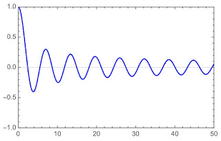
Really? Here’s a plot of J₀(x).

It oscillates like crazy and the envelope of those oscillations falls off very slowly. In fact, an asymptotic expansion for J₀ at large x is

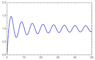
The leading factor of 1/√x decays so slowly that its integral from zero to infinity does not converge. Yet, when you include the cosine so the function oscillates, the integral does converge. Here’s a plot of

The integral approaches one at large x, but very slowly. So, the expression given in the problem is correct, but I sure wouldn’t want to do any numerical calculations using it, where I had to truncate the endpoint of the integral to something less than infinity. That would be a mess!

Here’s another interesting fact. Bessel functions come in many orders—J₀, J₁, J₂, etc.—and they all integrate to one.

Who’s responsible for these strangely-behaved functions? They’re named after the German astronomer Friedrich Bessel but they were first defined by the Swiss mathematician Daniel Bernoulli (1700–1782), a member of the brilliant Bernoulli family. The Bernoulli equation, mentioned in Chapter 1 of IPMB, is also named for Daniel Bernoulli. 

There was a time when I was in graduate school that I was obsessed with Bessel functions, especially modified Bessel functions that don’t oscillate. I’m not so preoccupied by them now, but they remain my favorite of the many special functions encountered in physics.

The Preface as Poetry

Alexander Pope

I mentioned before in this blog that I’m reading Will and Ariel Durant’s eleven-volume masterpiece The Story of Civilization. Recently, in Volume Nine about The Age of Voltaire, they discussed Alexander Pope, the eighteenth century English poet who, among other things, translated the Iliad into English poetry using iambic pentameter heroic couplets. Thus inspired, I decided to translate the preface of Intermediate Physics for Medicine and Biology from prose to poetry. I’d tell you to “Enjoy!” but I’m not sure that’ll be possible for such doggerel.

In the preface to the third edition, 

Russell Hobbie set out on a mission. 

For the two years before seventy three 

He audited the University

Of Minnesota’s medical courses. 

He found a lack of physics discourses. 

An intermediate physics class would 

For these students be so useful and good. 

This book is the result of when he taught 

Such a course that students needed a lot. 

He hoped that even those physics teachers 

Scared of bio would value its features. 

And doctors would find it a good reference 

With the physics concepts never too dense. 

Because the book was used by those whose tools 

From math were not vast he set down four rules: 

Calculus would be used without regret, 

And reviewed in detail when not seen yet. 

Readers should know the vocabulary 

But it’s told from the start, it’s not scary. 

He did not skip steps in derivations, 

And shunned any weirdo math notations. 

Hobbie added someone to help him write 

The Fourth Edition, and they did not fight. 

They wrote a new chapter, but made sure that 

The new edition did not get too fat. 

They added more than one homework problem, 

And a solution manual for them. 

Chapter One reviews biomechanics, 

Stress and strain, also fluid dynamics. 

Then Two discusses the exponential 

A math function that’s truly essential.

Next Three deals with temperature and heat, 

Biothermodynamics it does treat. 

Diffusion’s the topic of Chapter Four 

A random walk, and drift, and so much more. 

Chapter Five describes flow across membranes, 

And osmosis from ions that it contains. 

Six covers bioelectricity, 

And a model by Hodgkin and Huxley. 

Chapter Seven contains the EKG, 

And defibrillation is really key. 

Chapter Eight deals with all things magnetic, 

Interesting, but not too poetic. 

Nine begins with the model of Donnan, 

Then Nernst-Planck, Debye-Huckel, and so on. 

Chapter Ten has lots of mathematics, 

With feedback and chaos and dynamics. 

Eleven derives Fourier transforms.

Least squares and correlations, it brainstorms. 

Next Twelve analyzes tomography, 

Which allows you to image in 3D!

Chapter Thirteen considers ultrasound, 

A topic that you’ll find really profound. 

Next Chapter Fourteen summarizes light, 

Mix red and green and blue and you get white!

Fifteen considers photons and matter: 

Photoelectric and Compton Scatter. 

Chapter Sixteen is about the x-ray, 

Where the unit for dose is named the gray. 

Seventeen is about technetium, 

Nuclear medicine, and even then some. 

Then Eighteen is not about anything 

But magnetic resonance imaging. 

Biophysics is a subject quite broad, 

Of which we are always completely awed. 

Our book has grown and become large enough, 

To fit molecular stuff would be tough. 

We would like to get any corrections,

Or even hear about your suggestions. 

And last we thank our long-suffering wives, 

We know that this book disrupted their lives.

The Age of Voltaire,
by Will and Ariel Durant.

 The Iliad, translated by Alexander Pope (the heroic couplets start at 2:20).

https://www.youtube.com/watch?v=28RNGOCIzYI

 

Numerical Recipes is Online

Numerical Recipes,
by Press, Teukolsky, Vetterling, and Flannery.

In Intermediate Physics for Medicine and Biology, Russ Hobbie and I often refer to Numerical Recipes: The Art of Scientific Computing, by William Press, Saul Teukolsky, William Vetterling, and Brian Flannery. We usually cite the second edition of the book with programs written in C (1995), but the copy on my bookshelf is the second edition using Fortran 77 (1992). For those of you who don’t own a copy of this wonderful book, did you know you can read it online?

The address of the Numerical Recipes website is easy to remember: numerical.recipes. There you will find free copies of the second editions of Numerical Recipes for Fortran 77, Fortran 90, C, and C++ (2002). If you want easy, quick access to the third edition (2007), you will have to pay a fee. But if you are willing to put up with brief delays and annoying messages (which the authors call “nags”), you also can read the third edition for free.

The text below is from the Preface to the third edition.

“I was just going to say, when I was interrupted...” begins Oliver Wendell Holmes in the second series of his famous essays, The Autocrat of the Breakfast Table. The interruption referred to was a gap of 25 years. In our case, as the autocrats of Numerical Recipes, the gap between our second and third editions has been “only” 15 years. Scientific computing has changed enormously in that time.

The first edition of Numerical Recipes was roughly coincident with the first commercial success of the personal computer. The second edition came at about the time that the Internet, as we know it today, was created. Now, as we launch the third edition, the practice of science and engineering, and thus scientific computing, has been profoundly altered by the mature Internet and Web. It is no longer difficult to find somebody’s algorithm, and usually free code, for almost any conceivable scientific application. The critical questions have instead become, “How does it work?” and “Is it any good?” Correspondingly, the second edition of Numerical Recipes has come to be valued more and more for its text explanations, concise mathematical derivations, critical judgments, and advice, and less for its code implementations per se.

Recognizing the change, we have expanded and improved the text in many places in this edition and added many completely new sections. We seriously considered leaving the code out entirely, or making it available only on the Web. However, in the end, we decided that without code, it wouldn’t be Numerical Recipes. That is, without code you, the reader, could never know whether our advice was in fact honest, implementable, and practical. Many discussions of algorithms in the literature and on the Web omit crucial details that can only be uncovered by actually coding (our job) or reading compilable code (your job). Also, we needed actual code to teach and illustrate the large number of lessons about object-oriented programming that are implicit and explicit in this edition.

Russ and I cited Numerical Recipes in IPMB when we discussed integration, least squares fitting, random number generators, partial differential equations, the fast Fourier transform, aliasing, the correlation function, the power spectral density, and bilinear interpolation. Over the years, in my own research I have consulted the book about other topics, including solving systems of linear equations, evaluation of special functions, and computational analysis of eigensystems.

I highly recommend Numerical Recipes to anyone doing numerical computing. I found the book to be indispensable.

Is Shot Noise Also White Noise?

In Chapters 9 and 11 of Intermediate Physics for Medicine and Biology, Russ Hobbie and I discuss shot noise.

9.8.1 Shot Noise

The first (and smallest) limitation [on our ability to measure current] is called shot noise. It is due to the fact that the charge is transported by ions that move randomly and independently through the channels....

11.16.2 Shot Noise

Chapter 9 also mentioned shot noise, which occurs because the charge carriers have a finite charge, so the number of them passing a given point in a circuit in a given time fluctuates about an average value. One can show that shot noise is also white noise [my italics].

Introduction to Membrane Noise,
by Louis DeFelice

How does one show that shot noise is white noise (independent of frequency)? I’m going to follow Lou DeFelice’s explanation in his book Introduction to Membrane Noise (cited in IPMB). I won’t give a rigorous proof. Instead, I’ll first state Campbell’s theorem (without proving it), and then show that the whiteness of shot noise is a consequence of that theorem.

Campbell’s Theorem

To start, I’ll quote DeFelice, but I will change the names of a few variables.

Suppose N impulses i(t) arrive randomly in the time interval T. The sum of these will result in a random noise signal I(t). This is shown qualitatively in Figure 78.1.

Below is my version of Fig. 78.1.

A diagram illustrating the sum of N impulses, i(t), each shown in red, arriving randomly in the time interval T. The blue curve represents their sum, I(t), and the green dashed line represents the average, <I(t)>. Adapted from Fig. 78.1 in Introduction to Membrane Noise by Louis DeFelice.

DeFelice shows that the average of I(t), which I’ll denote <I(t)>, is

Here he lets T and N both be large, but their ratio (the average rate that the impulses arrived) remains finite.

He then shows that the variance of I(t), called σ_I², is

Finally, he writes

In order to calculate the spectral density of I(t) from i(t) we need Rayleigh’s theorem [also known as Parseval’s theorem]…

where î(f) is the Fourier transform of i(t) [and f is the frequency].

He concludes that the spectral density S_I(f) is given by

These three results (for the average, the variance, and the spectral density) constitute Campbell’s theorem.

Shot Noise

Now, let’s analyze shot noise by using Campbell’s theorem assuming the impulse is a delta function (zero everywhere except at t = 0 where it’s infinite). Set i(t) = q δ(t), where q is the charge of each discrete charge carrier.

First, the average <I(t)> is simply Nq/T, or the total charge divided by the total time. 

Second, the variance is the integral of the delta function squared. When any function is multiplied by a delta function and then integrated over time, you get that function evaluated at time zero. So, the integral of the square of the delta function gives the delta function itself evaluated at zero, which is infinity. Yikes! The variance of shot noise is infinite.

Third, to get the spectral density of shot noise we need the Fourier transform of the delta function. 

The key point is that S_I(f) is independent of frequency; it’s white.

DeFelice ends with

This [the expression for the spectral density] is the formula for shot noise first derived by Schottky (1918, pp. 541-567) in 1918. Evidently, the variance defined as

is again infinite; this is a consequence of the infinitely small width of the delta function.

As DeFelice reminds us, shot noise is white because the delta function is infinitely narrow. As soon as you assume i(t) has some width (perhaps the time it takes for a charge to cross the membrane), the spectrum will fall off at high frequencies, the variance won’t be infinite (thank goodness!), and the noise won’t be white. The bottom line is that shot noise is white because the Fourier transform of a delta function is a constant.

Conclusion

Perhaps you’re thinking I haven’t helped you all that much. I merely changed your question from “why is shot noise white” to “how do I prove Campbell’s theorem.” You have a point. Maybe proving Campbell’s theorem can be the story of another post.

I met Lou DeFelice in 1984, when I was a graduate student at Vanderbilt University and he came to give a talk. In the summer of 1986, my PhD advisor John Wikswo and I traveled to Emory University to visit DeFelice and Robert DeHaan. During that trip, Wikswo and I were walking across the Emory campus when Wikswo decided he knew a short cut (he didn’t). He left the sidewalk and entered a forest, with me following behind him. After what seemed like half an hour of wandering through a thicket, we emerged from the woods at a back entrance to the Yerkes Primate Research Center. We’re lucky we weren’t arrested.

DeFelice joined the faculty at Vanderbilt in 1995, and we both worked there in the late 1990s. He was a physicist by training, but spent most of his career studying electrophysiology. Sadly, in 2016 he passed away.

The Central Slice Theorem: An Example

The central slice theorem is key to understanding tomography. In Intermediate Physics for Medicine and Biology, Russ Hobbie and I ask the reader to prove the central slice theorem in a homework problem. Proofs are useful for their generality, but I often understand a theorem better by working an example. In this post, I present a new homework problem that guides you through every step needed to verify the central slice theorem. This example contains a lot of math, but once you get past the calculation details you will find it provides much insight.

The central slice theorem states that taking a one-dimensional Fourier transform of a projection is equivalent to taking the two-dimensional Fourier transform and evaluating it along one direction in frequency space. Our “object” will be a mathematical function (representing, say, the x-ray attenuation coefficient as a function of position). Here is a summary of the process, cast as a homework problem.

Section 12.4 

Problem 21½. Verify the central slice theorem for the object

(a) Calculate the projection of the object using Eq. 12.29,

Then take a one-dimensional Fourier transform of the projection using Eq. 11.59,

 

(b) Calculate the two-dimensional Fourier transform of the object using Eq. 12.11a,

Then transform F̂(k_x,k_y ) to F̂(θ,k) by converting from Cartesian to polar coordinates in frequency space.

(c) Compare your answers to parts (a) and (b). Are they the same?

I’ll outline the solution to this problem, and leave it to the reader to fill in the missing steps. 

 

Fig. 12.12 from IPMB, showing how to do a projection.

The Projection 

Figure 12.12 shows that the projection is an integral of the object along various lines in the direction θ, as a function of displacement perpendicular to each line, x'. The integral becomes

Note that you must replace x and y by the rotated coordinates x' and y'

You can verify that x² + y²= x'² + y'².

After some algebra, you’re left with integrals involving e^−by'2 (Gaussian integrals) such as those analyzed in Appendix K of IPMB. The three you’ll need are

The resulting projection is

Think of the projection as a function of x', with the angle θ being a parameter.

 

The One-Dimensional Fourier Transform

The next step is to evaluate the one-dimensional Fourier transform of the projection

The variable k is the spatial frequency. This integral isn’t as difficult as it appears. The trick is to complete the square of the exponent

Then make a variable substitution u = x' + ik⁄2b. Finally, use those Gaussian integrals again. You get

This is our big result: the one-dimensional Fourier transform of the projection. Our next goal is to show that it’s equal to the two-dimensional Fourier transform of the object evaluated in the direction θ.

Two-Dimensional Fourier Transform

To calculate the two-dimensional Fourier transform, we must evaluate the double integral

The variables k_x and k_y are again spatial frequencies, and they make up a two-dimensional domain we call frequency space.

You can separate this double integral into the product of an integral over x and an integral over y. Solving these requires—guess what—a lot of algebra, completing the square, and Gaussian integrals. But the process is straightforward, and you get

Select One Direction in Frequency Space

If we want to focus on one direction in frequency space, we must convert to polar coordinates: k_x = k cosθ and k_y = k sinθ. The result is 

This is exactly the result we found before! In other words, we can take the one-dimensional Fourier transform of the projection, or the two-dimensional Fourier transform of the object evaluated in the direction θ in frequency space, and we get the same result. The central slice theorem works.

I admit, the steps I left out involve a lot of calculations, and not everyone enjoys math (why not?!). But in the end you verify the central slice theorem for a specific example. I hope this helps clarify the process, and provides insight into what the central slice theorem is telling us.

Projections and Filtered Projections of a Square

Chapter 12 of Intermediate Physics for Medicine and Biology describes tomography. Russ Hobbie and I write

The reconstruction problem can be stated as follows. A function f(x,y) exists in two dimensions. Measurements are made that give projections: the integrals of f(x,y) along various lines as a function of displacement perpendicular to each line. For example, integration parallel to the y axis gives a function of x,

as shown in Fig. 12.12. The scan is repeated at many different angles θ with the x axis, giving a set of functions F(θ, x'), where x' is the distance along the axis at angle θ with the x axis.

One example in IPMB is the projection of a simple object: the circular top-hat

The projection can be calculated analytically

It’s independent of θ; it looks the same in every direction.

Let’s consider a slightly more complicated object: the square top-hat

This projection can be found using high school geometry and trigonometry (evaluating it is equivalent to finding the length of lines passing through the square at different angles). I leave the details to you. If you get stuck, email me (roth@oakland.edu) and I’ll send a picture of some squares and triangles that explains it.

The plot below shows the projections at four angles. For θ = 0° the projection is a rectangle; for θ = 45° it’s a triangle, and for intermediate angles (θ = 15° and 30°) it’s a trapezoid. Unlike the circular top-hat, the projection of the square top-hat depends on the direction.

The projections of a square top-hat, at different angles.

What I just described is the forward problem of tomography: calculating the projections from the object. As Russ and I wrote, usually the measuring device records projections, so you don’t have to calculate them. The central goal of tomography is the inverse problem: calculating the object from the projections. One way to perform such a reconstruction is a two-step procedure known as filtered back projection: first high-pass filter the projections and then back project them. In a previous post, I went through this entire procedure analytically for a circular top-hat. Today, I go through the filtering process analytically, obtaining an expression for the filtered projection of a square top-hat. 

Here we go. I warn you, there’s lots of math. To perform the filtering, we first calculate the Fourier transform of the projection, C_F(θ,k). Because the top-hat is even, we can use the cosine transform

where k is the spatial frequency.

Next, place the expression for F(θ,x') into the integral and evaluate it. There’s plenty of book-keeping, but the projection is either constant or linear in x', so the integrals are straightforward. I leave the details to you; if you work it out yourself, you’ll be delighted to find that many terms cancel, leaving the simple result 

To high-pass filter C_F(θ,k), multiply it by |k|/2π to get the Fourier transform of the filtered projection C_G(θ,k)

Finally, take the inverse Fourier transform to obtain the filtered projection G(θ,x') 

Inserting our expression for C_G(θ,k), we find

This integral is not trivial, but with some help from WolframAlpha I found

where Ci is the cosine integral. I admit, this is a complicated expression. The cosine integral goes to zero for large argument, so the upper limit vanishes. It goes to negative infinity logarithmically at zero argument. We’re in luck, however, because the four cosine integrals conspire to cancel all the infinities, allowing us to obtain an analytical expression for the filtered projection

We did it! Below are plots of the filtered projections at four angles. 

The filtered projections of a square top-hat, at different angles.

The last thing to do is back project G(θ,x') to get the object f(x,y). Unfortunately, I see no hope of back-projecting this function analytically; it’s too complicated. If you can do it, let me know.

Why must we analyze all this math? Because solving a simple example analytically provides insight into filtered back projection. You can do tomography using canned computer code, but you won’t experience the process like you will by slogging through each step by hand. If you don’t buy that argument, then another reason for doing the math is: it’s fun!