Showing posts with label new homework problem. Show all posts

Friday, December 7, 2018

Imaging and Velocimetry of the Human Retinal Circulation with Color Doppler Optical Coherence Tomography

Page 394 of Intermediate Physics for Medicine and Biology.
Page 394 of IPMB.
Section 14.7 of Intermediate Physics for Medicine and Biology discuses optical coherence tomography (OCT). Russ Hobbie and I write
Optical range measurements using the time delay of reflected or backscattered light from pulses of a few femtosecond (10-15 s) duration can be used to produce images similar to those of ultrasound…Since it is difficult to measure time intervals that short, most measurements are done using interference properties of the light. Optical coherence tomography is conceptually similar to range measurements but uses interference measurements…It is widely used in ophthalmology….
Intermediate Physics for Medicine and Biology Fig. 14.15.
Fig. 14.15 of IPMB.
The basic apparatus [for OCT] is shown in Fig. 14.15….The light pulse travels over an optical fiber to a 50/50 beam splitter. Part travels to the sample, where it is reflected back to the 50/50 coupler and then to the detector. The other half of the light goes to the reference mirror, where it is also reflected back to the detector. Changing the position of the reference mirror changes the depth of the image plane in the sample….

Intermediate Physics for Medicine and Biology Fig. 14.17.
Fig. 14.17 of IPMB.
It is possible to make many kinds of images. Fig. 14.17 shows the parabolic velocity profile of blood flowing in a retinal blood vessel 176 μm diameter. It was obtained by measuring the Doppler shift in light scattered from moving blood cells.
Yazdanfar et al. (2000).
Figure 14.17 is from the paper “Imaging and Velocimetry of the Human Retinal Circulation with Color Doppler Optical Coherence Tomography,” by Siavash Yazdanfar, Andrew Rollins, and Joseph Izatt (Optical Letters, Volume 25, Pages 1448–1450, 2000). [For some reason Russ and I did not include the year in our citation—another item for the errata].
Abstract: Noninvasive monitoring of blood flow in retinal microcirculation may elucidate the progression and treatment of ocular disorders, including diabetic retinopathy, age-related macular degeneration, and glaucoma. Color Doppler optical coherence tomography (CDOCT) is a technique that allows simultaneous micrometer-scale resolution cross-sectional imaging of tissue microstructure and blood flow in living tissues. CDOCT is demonstrated for the first time in living human subjects for bidirectional blood-flow mapping of retinal vasculature.
I like Fig 14.17 because it combines ideas from Chapters 1, 11, 13, and 14 of IPMB. It also highlights the excellent spatial resolution you can obtain with OCT.

The illustration below shows the geometry associated with Fig. 14.17. The light is reflected by blood cells moving at speed v, causing a Doppler shift in its frequency. By adjusting the reference mirror, different depths are selected. The vessel makes an angle θ relative to the incident light. As the depth is scanned across the vessel, the Doppler shift determines the blood flow profile.
The geometry associated with Intermediate Physics for Medicine and Biology, Fig. 14.17.
The geometry associated with IPMB Fig. 14.17.
To help the reader learn more about the physics of OCT and Fig. 14.17, I have written two new homework problems. The solutions are included at the bottom of the post (upside down, to encourage readers to solve the problems themselves first). Enjoy!
Section 14.7

Problem 24 ⅓. This problem and the next explore the physics behind Fig. 14.17, which shows the velocity profile in a blood vessel measured using color Doppler optical coherence tomography. The data is based on an article by Yazdanfar et al. (2000). For this problem ignore the index of refraction of the tissue and assume θ = 60°.

(a) If the wavelength, λ, of the incident light is 832 nm and the wavelength bandwidth, Δλ, is 15 nm, determine the frequency, f, and the frequency bandwidth, Δf, in THz.

(b) The coherence time, τcoh, is equal to 1/(πΔf). Calculate τcoh in fs, and the coherence length, x2x1, in microns. The coherence length determines the spatial resolution of the measurement.

(c) Use Eq. 13.42 to derive an expression for the speed of blood flow in the direction of the light, v', in terms of the Doppler frequency shift, df. Assume that the speed of light, c, is much greater than v'. Calculate v' if df = 4 kHz. The Doppler technique measures the component of motion in the direction of the light. Determine the speed v along the vessel.

Problem 24 ⅔. The Doppler shift, df, of OCT data as a function of depth z across a blood vessel is given below. For viscous flow in a tube (Sec. 1.17), the blood speed varies parabolically across the vessel cross section (Eq. 1.37). Fit a parabola to this data of the form df = Az2 + Bz + C, and determine constants A, B, and C. Use these constants to find the peak value of df in this vessel, the location of the center of the vessel, and the vessel diameter (the width of the parabola when df = 0). The measured diameter corresponds to an oblique section at θ = 60°. Correct this result to get the true diameter.
   z (mm)    df (kHz)
0.15 3.26
0.20 5.20
0.25 6.12
0.30 6.02
0.35 4.89
0.40 2.75
I will give the final word to Yazdanfar, Rollins, and Izatt, who conclude
In summary, CDOCT has been applied for what is believed to be the first time to retinal blood-flow mapping in the human eye. Depth-resolved quantification of retinal hemodynamics may prove helpful in understanding the pathogenesis of several ocular diseases. Unlike fluorescein angiography, CDOCT is entirely noninvasive and does not require dilation of the pupil. Furthermore, CDOCT operates at longer wavelengths than does laser Doppler velocimetry, so light exposure times can be safely increased. CDOCT is believed to be the first technique for determining, with micrometer-scale resolution, the depth, diameter, and flow rate of blood vessels within the living retina.
Solution to new Homework Problem 24 ⅓
Solution to new Homework Problem 24 ⅔.

Friday, October 12, 2018

A Trick to Generate Exam Problems

Intermediate Physics for Medicine and Biology.
When teaching a class based on Intermediate Physics for Medicine and Biology, instructors need to write problems for their exams. My goal in this post is to explain a trick for creating good exam problems. 

One of my favorite homework problems in IPMB is from Chapter 4.
Problem 37. The goal of this problem is to estimate how large a cell living in an oxygenated medium can be before it is limited by oxygen transport. Assume the extracellular space is well stirred with uniform oxygen concentration C0. The cell is a sphere of radius R. Inside the cell oxygen is consumed at a rate Q molecule m−3 s−1. The diffusion constant for oxygen in the cell is D.
(a) Calculate the concentration of oxygen in the cell in the steady state.
(b) Assume that if the cell is to survive the oxygen concentration at the center of the cell cannot become negative. Use this constraint to estimate the maximum size of the cell.
(c) Calculate the maximum size of a cell for C0 = 8 mol m−3, D = 2 x 10⁻⁹ m2 s−1, Q = 0.1 mol m−3 s−1. (This value of Q is typical of protozoa; the value of C0 is for air and is roughly the same as the oxygen concentration in blood.)
Homework problems for Chapter 4 in Intermediate Physics for Medicine and Biology.
Homework problems for Chapter 4 in
Intermediate Physics for Medicine and Biology.
I usually work this problem in class. Not only do students practice solving the steady-state diffusion equation, but also they estimate the maximum size of a cell from some basic properties of oxygen. In the Solution Manual—available to instructors only (email us)—we explain the purpose of each problem in a preamble. Here is what the solution manual says about Problem 37:
This important “toy model” considers the maximum size of a spherical cell before its core dies from lack of oxygen. One goal of biological physics is to show how physics constrains evolution. In this case, the physics of diffusion limits how large an animal can be before needing a circulatory system to move oxygen around.
How do you create an exam problem on this subject? Here's the trick: Do Problem 37 in class and then put a question on the exam identical to Problem 37 except “sphere” is replaced by “cylinder”. The problem is only slightly changed; just enough to determine if the student is solving the problem from first principles or merely memorizing. In addition, nerve and muscle fibers are cylindrical, so the revised problem may provide an even better model for those cells. Depending on the mathematical abilities of your students, you may need to provide students with the Laplacian in cylindrical coordinates. (If the exam is open book then they can find the Laplacian in Appendix L).

Here’s a second example: Chapter 1 considers viscous flow in a tube; Poiseuille flow. On the exam, ask the student to analyze viscous flow between two stationary plates.
Section 1.17
Problem 36 ½. Consider fluid flow between two stationary plates driven by a pressure gradient. The pressure varies in the x direction with constant gradient dp/dx, the plates are located at y = +L and y = -L, and the system is uniform in the z direction with width H. The fluid has viscosity η.

(a) Draw a picture the geometry.
(b) Consider a rectangular box of fluid centered at the origin and derive a differential equation like Eq. 1.35 governing the velocity vx(y).

(c) Solve this differential equation to determine vx(y), analogous to Eq. 1.37. Assume a no-slip boundary condition at the surface of each plate. Plot vx(y) versus y.

(d) Integrate the volume fluence and find the total flow i. How does i depend on the plate separation, 2L? How does this compare with the case of flow in a tube?
An interesting feature of this example is that i depends on the third power of L, whereas for a tube it depends on the fourth power of the radius. Encourage the student to wonder why.

Third example: A problem in Chapter 7 compares three different functions describing the strength-duration curve for electrical stimulation. On your exam, have the students analyze a fourth case.
Section 7.10

Problem 46 ½. Problem 46 analyzes three possible functions that could describe the strength-duration curve, relating the threshold current strength required for neural excitation, i, to the stimulus pulse duration, t. Consider the function i = A/tan-1(t/B). Derive expressions for the rheobase iR and chronaxie tC in terms of A and B. Write the function in the form used in Problem 46. Plot i versus t.
And still more: Problem 32 in Chapter 8 examines magnetic stimulation of a nerve axon using an applied electric field Ei(x) = E0 a2/(x2 + a2). Give a similar problem on your exam but use a different electric field, such as Ei(x) = E0 exp(-x2/a2).

And yet another: Chapter 10 examines the onset of cardiac fibrillation and chaos. The action potential duration APD is related to the diastolic interval (time from the end of the previous action potential to the start of the following one) DI by the restitution curve. Have the student repeat Problem 41 but using a different restitution curve: APDi+1 = 300 DIi/(DIi + 100).

Final example: Problem 36 in Chapter 9 asks the student to calculate the electrical potential inside and outside a spherical cell in the presence of a uniform electric field (Figure 9.19). On your exam, make the sphere into a cylinder.

I think you get the point. On an exam, repeat one the of homework problems in IPMB, but with a twist. Change the problem slightly, using a new function or a modified geometry. You will be able to test the knowledge and understanding of the student without springing any big surprises on the exam. Many problems in IPMB that could be modified in this way.

Warning: This trick doesn’t always work. For instance, in Chapter 1 if you try to analyze fluid flow perpendicular to a stationary object, you run into difficulties when you change the sphere of Problem 46 into a cylinder. The cylindrical version of this problem has no solution! The lack of a solution for low Reynolds number flow around a cylinder is known as Stokes’ Paradox. In that case, you’re just going to have to think up your own exam question.

Friday, October 5, 2018

A Bidomain Model for the Extracellular Potential and Magnetic Field of Cardiac Tissue

My research notebooks from graduate school.
In graduate school, I worked with John Wikswo measuring the 
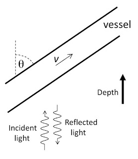
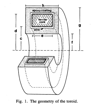
magnetic field of a nerve axon. We isolated a crayfish axon and threaded it through a wire-wound ferrite-core toroid immersed in saline. As the action currents propagated by, they produced a changing magnetic field that induced a signal in the toroid by Faraday induction. Ampere’s law tells us that the signal is proportional to the net current through the toroid, which is the sum of the intracellular current and the fraction of the current in the saline that passes through the toroid, called the return current.

For my PhD dissertation, Wikswo had me make similar measurements on strands of cardiac tissue, such as a 
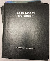
papillary muscle. The instrumentation was the same as for the nerve, but the interpretation was different. Now the signal had three sources: the intracellular current, the return current in the saline, and extracellular current passing through the interstitial space within the muscle called the “interstitial return current.” Initially neither Wikswo nor I knew how to calculate the interstitial return current, so we were not sure how to interpret our results. As I planned these experiments, I recorded my thoughts in my research notebook. The July 26, 1984 entry stressed that “Understanding this point [the role of interstitial return currents] will be central to my research and deserves much thought.”

Excerpt from the July 26, 1984 entry in my Notebook 8, page 64.
When working on nerves, I had studied articles by Robert Plonsey and John Clark, in which they calculated the extracellular potential in the saline from the measured voltage across the axon’s membrane: the transmembrane potential. I was impressed by this calculation, which involved Fourier transforms and Bessel functions (see Chapter 7, Problem 30, in Intermediate Physics for Medicine and Biology). I had used their result to calculate the magnetic field around an axon (see Chapter 8, Problem 16 in IPMB), so I set out to extend their analysis again to include interstitial return currents.

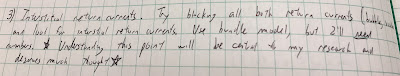
Page 1 of Notebook 9, from Sept 13, 1984.
The key was to use the then-new bidomain model, which accounts for currents in both the intracellular and interstitial spaces. The crucial advance came in September 1984 after I read a copy of Les Tung’s PhD dissertation that Wikswo had loaned me. After four days of intense work, I had solved the problem. My results looked a lot like those of Clark and Plonsey, except for a few strategically placed additional factors and extra terms.
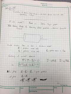
Excerpt from Notebook 9, page 13, the Sept 16, 1984 entry.
First page of Roth and Wikswo (1986) IEEE Trans. Biomed. Eng., 33:467–469.
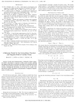
First page of Roth and Wikswo (1986).
Wikswo and I published these results as a brief communication in the IEEE Transactions on Biomedical Engineering.
Roth, B. J. and J. P. Wikswo, Jr., 1986, A bidomain model for the extracellular potential and magnetic field of cardiac tissue. IEEE Trans. Biomed. Eng., 33:467-469.

Abstract—In this brief communication, a bidomain volume conductor model is developed to represent cardiac muscle strands, enabling the magnetic field and extracellular potential to be calculated from the cardiac transmembrane potential. The model accounts for all action currents, including the interstitial current between the cardiac cells, and thereby allows quantitative interpretation of magnetic measurements of cardiac muscle.
Rather than explain the calculation in all its gory detail, I will ask you to solve it in a new homework problem.
Section 7.9
Problem 31½. A cylindrical strand of cardiac tissue, of radius a, is immersed in a saline bath. Cardiac tissue is a bidomain with anisotropic intracellular and interstitial conductivities σir, σiz, σor, and σoz, and saline is a monodomain volume conductor with isotropic conductivity σe. The intracellular and interstitial potentials are Vi and Vo, and the saline potential is Ve.
a) Write the bidomain equations, Eqs. 7.44a and 7.44b, for Vi and Vo in cylindrical coordinates (r,z). Add the two equations.
b) Assume Vi = σiz/(σiz+σoz) [A I0(kλr) + (σoz/σiz) Vm] sin(kz) and Vo = σiz/(σiz+σoz) [A I0(kλr) - Vm] sin(kz) where λ2 = (σiz+σoz)/(σir+σor). Verify that Vi - Vo equals the transmembrane potential Vm sin(kz). Show that Vi and Vo obey the equation derived in part a). I0(x) is the modified Bessel function of the first kind of order zero, which obeys the modified Bessel equation d2y/dx2 + (1/x) dy/dx = y. Assume Vm is independent of r.
c) Write Laplace’s equation (Eq. 7.38) in cylindrical coordinates. Assume Ve = B K0(kr) sin(kz). Show that Ve satisfies Laplace’s equation. K0(x) is the modified Bessel function of the second kind of order zero, which obeys the modified Bessel equation.
d) At r = a, the boundary conditions are Vo = Ve and σirVi/∂r + σorVo/∂r = σeVe/∂r. Determine A and B. You may need the Bessel function identities dI0/dx = I1 and dK0/dx = - K1, where I1(x) and K1(x) are modified Bessel functions of order one.
In the problem above, I assumed the potentials vary sinusoidally with z, but any waveform can be expressed as a superposition of sines and cosines (Fourier analysis) so this is not as restrictive as it seems.

In part b), I assumed the transmembrane potential was not a function of r. There is little data supporting this assumption, but I was stuck without it. Another assumption I could have used was equal anisotropy ratios, but I didn’t want to do that (and initially I didn’t realize it provided an alternative path to the solution).

The calculation of the magnetic field is not included in the new problem; it requires differentiating Vi, Vo, and Ve to find the current density, and then integrating the current to find the magnetic field via Ampere’s law. You can find the details in our IEEE TBME communication.

Some of you might be thinking “this is a nice homework problem, but how did you get those weird expressions for the intracellular and interstitial potentials used in part b)”? Our article gives some insight, and my notebook provides more. I started with Clark and Plonsey’s result, used ideas from Tung’s dissertation, and then played with the math (trial and error) until I had a solution that obeyed the bidomain equations. Some might call that a strange way to do science, but it worked for me.

I was very proud of this calculation (and still am). It played a role in the development of the bidomain model, which is now considered the state-of-the-art model for simulating the heart during defibrillation.

Wikswo and I carried out experiments on guinea pig papillary muscles to test the calculation, but the cardiac data was not as clean and definitive as our nerve data. We published it as a chapter in Cell Interactions and Gap Junctions (1989). The cardiac work made up most of my PhD dissertation. Vanderbilt let me include our three-page IEEE TBME communication as an appendix. It’s the most important three pages in the dissertation.


Coda: While browsing through my old research notebooks, I found this gem passed from Prof. Wikswo to his earnest but naive graduate student, who dutifully wrote it down in his research notebook for posterity.

Excerpt from Notebook 10, Page 62, January 3, 1985.
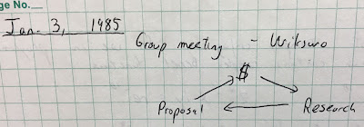
Excerpt from Notebook 10, Page 62.

Friday, March 30, 2018

The Radiation Dose from Radon: A Back-of-the-Envelope Estimation

Intermediate Physics for Medicine and Biology: The Radiation Dose from Radon I like Fermi problems: those back-of-the-envelope order-of-magnitude estimates that don’t aim for accuracy, but highlight underlying principles. I also enjoy devising new homework exercises for the readers of this blog. Finally, I am fascinated by radon, that radioactive gas that contributes so much to the natural background radiation. Ergo, I decided to write a new homework problem about estimating the radiation dose from breathing radon.

What a mistake. The behavior of radon is complex, and the literature is complicated and confusing. Part of me regrets starting down this path. But rather than give up, I plan to forge ahead and to drag you—dear reader—along with me.
Section 17.12
Problem 57 1/2. Estimate the annual effective dose (in Sv yr-1) if the air contains a trace of radon. Use the data in Fig. 17.27, and assume the concentration of radon corresponds to an activity of 150 Bq m-3, which is the action level at which the Environmental Protection Agency suggests you start to take precautions. Make reasonable guesses for any parameters your need.
Here is my solution (stop reading now if you first want to solve the problem yourself). In order to be accessible to a wide audience, I avoid jargon and unfamiliar units.
One bequerel is a decay per second, and a cubic meter is 1000 liters, so we start with 0.15 decays per second per liter. The volume of air in your lungs is about 6 liters, implying that approximately one atom of radon decays in your lungs every second.

Radon decays by emitting an alpha particle. You don’t, however, get just one. Radon-222 (the most common isotope of radon) alpha-decays to polonium-218, which alpha-decays to lead-214, which beta-decays twice to polonium-214, which alpha-decays to lead-210 (see Fig 17.27 in Intermediate Physics for Medicine and Biology). The half-life of lead-210 is so long (22 years) that we can treat it as stable. Each decay of radon therefore results in three alpha particles. An alpha particle is ejected with an energy of about 6 MeV. Therefore, roughly 18 MeV is deposited into your lungs each second. If we convert to SI units (1 MeV = 1.6 × 10⁻¹³ joule), we get about 3 × 10-12 joules per second.

Absorbed dose is expressed in grays, and one gray is a joule per kilogram. The mass of the lungs is about 1 kilogram. So, the dose rate for the lungs is 3 × 10-12 grays per second. To find the annual dose, multiply this dose rate by one year, or 3.2 × 10⁷ seconds. The result is about 10-4 gray, or a tenth of a milligray per year.

If you want the equivalent dose in sieverts, multiply the absorbed dose in grays by 20, which is the radiation weighting factor for alpha particles. To get the effective dose, multiply by the tissue weighting factor for the lungs, 0.12. The final result is 0.24 mSv per year.
This all seems nice and logical, except the result is a factor of ten too low! It is probably even worse than that, because my initial radon concentration was higher than average and in Table 16.6 of IPMB Russ Hobbie and I report a value of 2.28 mSv for the average annual effective dose. My calculation here is an estimate, so I don’t expect the answer to be exact. But when I saw such a low value I was worried and started to read some of the literature about radon dose calculations. Here is what I learned:
  1. The distribution of radon progeny (such as 214Po) is complicated. These short-lived isotopes are charged and behave differently than an unreactive noble gas like radon. They stick to particles in the air. Your dose depends on how dusty the air is.
  2. How these particles interact with our lungs is even more difficult to understand. Some large particles are filtered out by the upper respiratory track
  3. The range of a 6-MeV alpha particle is only about 50 microns, so some of the energy is deposited harmlessly into the gooey mucus layer lining the airways (see https://www.ncbi.nlm.nih.gov/books/NBK234233). Ironically, if you get bronchitis your mucus layer thickens, protecting you from radon-induced lung cancer.  
  4. The progeny and their dust particles stick to the bronchi walls like flies to flypaper, increasing their concentration.
  5. Filtering out dust and secreting a mucus layer reduces the dose to the lungs, while attaching the progeny to the airway lining increases it. My impression from the literature is that the flypaper effect dominants, and explains why my estimate is so low.
  6. The uranium-238 decay chain shown in Fig. 17.27 is the source of radon-222, but other isotopes arise from other decay chains. The thorium-232 decay chain leads to radon-220, called thoron, which also contributes to the dose.
  7. I am not confident about my value for the mass. The lungs are a bloody organ; about half of their mass is blood. I don’t know whether or not the blood is included in the reported 1 kg mass. The radon literature is oddly silent about the lung mass, and I don’t know how these authors calculate the dose without it. 
  8. I ignored the energy released when progeny beta-decay, which would cause a significant error if my aim was to calculate the absorbed dose in grays. But if I want the effective dose in sieverts I should be alright, because the radiation weighting factor for electrons is 1 compared to 20 for alpha particles. 
  9. The radon literature is difficult to follow in part because of strange units, such as picocuries per liter and working level months (see https://www.ncbi.nlm.nih.gov/books/NBK234224).
  10. Radon can get into the water as well as the air. If you drink the water, your stomach gets a dose. With a half-life of days, the radon in this elixir has time to enter your blood and irradiate your entire body.
  11. Does the dose from radon lead to lung cancer? That depends on the accuracy of the linear no-threshold model. If there is a threshold, then such a small dose may not represent a risk.
  12. If you want to learn more about radon, read NCRP Report 160, ICRP Publication 103, or BEIR VI. Of course, you should start by reading Section 17.12 in IPMB.
What do I take away from this estimation exercise? First, radon dosimetry is complicated. Second, biology problems are messy, and while order-of-magnitude estimates are still valuable, your results need large error bars.

Friday, February 2, 2018

Gauss and the Method of Least Squares

Intermediate Physics for Medicine and Biology: Gauss and the Method of Least Squares
Asimov's Biographical Encyclopedia of Science and Technology, by Isaac Asimov, superimposed on Intermediate Physics for Medicine and Biology.
Asimov’s Biographical Encyclopedia
of Science and Technology,
by Isaac Asimov.
In Chapter 11 of Intermediate Physics for Medicine and Biology, Russ Hobbie and I discuss fitting data using the method of least squares. This technique was invented by mathematicians Adrien Marie Legendre and Johann Karl Friedrich Gauss. Isaac Asimov describes Gauss’s contributions in Asimov’s Biographical Encyclopedia of Science and Technology.
While still in his teens he [Gauss] made a number of remarkable discoveries, including the method of least squares, advancing the work of Legendre in this area. By this [technique] the best equation for a curve fitting a group of observations can be made. Personal error is minimized. It was work such as this that enabled Gauss, while still in his early twenties, to calculate the orbit for [the asteroid] Ceres.
Of Time and Space and Other Things, by Isaac Asimov, superimposed on Intermediate Physics for Medicine and Biology.
Of Time and Space and Other Things,
by Isaac Asimov.
Asimov tells the story of Ceres in more detail in Of Time and Space and Other Things
Giuseppe Piazzi, an Italian astronomer … discovered, on the night of January 1, 1801, a point of light which had shifted its position against the background of stars. He followed it for a period of time and found it was continuing to move steadily. It moved less rapidly than Mars and more rapidly than Jupiter, so it was very likely a planet in an intermediate orbit …

Piazzi didn't have enough observations to calculate an orbit and this was bad. It would take months for the slow-moving planet to get to the other side of the Sun and into observable position, and without a calculated orbit it might easily take years to rediscover it.

Fortunately, a young German mathematician, Karl Friedrich Gauss, was just blazing his way upward into the mathematical firmament. He had worked out something called the “method of least squares,” which made it possible to calculate a reasonably good orbit from no more than three good observations of a planetary position.

Gauss calculated the orbit of Piazzi's new planet, and when it was in observable range once more there was [Heinrich] Olbers [a German astronomer] and his telescope watching the place where Gauss's calculations said it would be. Gauss was right and, on January 1, 1802, Olbers found it.
What is the role for least-squares fitting in medicine and biology? In many cases you want to fit experimental data to a mathematical model, in order to determine some unknown parameters. One example is the linear-quadratic model of radiation damage, presented in Chapter 16 of IPMB. Below is a new homework problem, designed to provide practice using the method of least squares to analyze data on cell survival during radiation exposure.
Section 16.9

Problem 29 ½. The fraction of cell survival, Psurvival, as a function of radiation dose, D (in Gy), is
D Psurvival
  0   1.000
  2   0.660
  4   0.306
  6   0.100
  8   0.0229
10   0.0037
Fit this data to the linear-quadratic model, Psurvival = eD – βD2 (Eq. 16.29) and determine the best-fit values of α and β. Plot Psurvival versus D on semilog graph paper, indicating the data points and a curve corresponding to the model. Hint: use the least-squares method outlined in Sec. 11.1, and make this into a linear least squares problem by taking the natural logarithm of Psurvival.
Gauss is mentioned often in IPMB. Section 6.3 discusses Gauss’s law relating the electric field to charge, and Appendix I discusses the Gaussian probability distribution (the normal, or bell-shaped curve). Asimov writes
Gauss…was an infant prodigy in mathematics who remained a prodigy all his life. He was capable of great feats of memory and of mental calculation…. Some people consider him to have been one of the three great mathematicians of all time, the others being Achimedes and Newton.

Friday, January 26, 2018

The Viscous Torque on a Rotating Sphere

Intermediate Physics for Medicine and Biology: The Viscous Torque on a Rotating Sphere In Section 9.10 of Intermediate Physics for Medicine and Biology, Russ Hobbie and I write
We saw in Chap. 4 (Stokes' law) that the translational viscous drag on a spherical particle is 6πηav. Similarly, the viscous torque on a rotating sphere is 8πηa3(dθ/dt).
Let’s calculate this torque. We always learn something when we see where such a result comes from.

To begin, we will redo Homework Problem 46 from Chapter 1 that asks you to calculate the translational Stokes’ law by considering a stationary sphere in a moving viscous fluid (equivalent to a sphere moving through a stationary viscous fluid). Below is the analogous problem for a sphere rotating in the same fluid.
Problem 46 ½. Consider a sphere of radius a rotating with angular velocity ω in a fluid of viscosity η. For low Reynolds number flow, the fluid velocity and pressure surrounding the sphere are

          vφ = ω a3 sinθ/r2

          vr = vθ = p = 0.

(a) Show that the no-slip boundary condition is satisfied.
(b) Integrate the shear torque over the sphere surface and find an expression for the net viscous torque on the sphere.
When I first tried to solve part (b), I kept getting an answer that was off by a factor of 2/3. I checked my work several times, but I couldn’t find any mistake. After much fussing, I finally figured out my error. For the shear stress at the sphere surface, I was using η dvφ/dr. This seemed right at first, but it’s not. The shear stress is actually η (dvφ/drvφ/r). Why? I could just say that I looked up the expression for the shear strain ε for spherical coordinates and found it had two terms. But that’s no fair (and no fun). We have to understand what we are doing, not just look things up. Why does the expression for the shear stress have two terms?

Let’s start on page 16 of IPMB, where Russ and I note that the shear stress is the viscosity times the rate of change of the shear strain. We need to see how the shear strain changes with time. There are two cases.
1. The first case will give us the familiar dv/dr expression for the shear stress. Consider an element of fluid with thickness dr, as shown below.
The velocity is in the φ direction, and depends on r. In time T, the top surface of the box moves to the right a distance vφ(r+dr) T, while the bottom surface moves only vφ(r) T, forming the dashed box in the figure. The shear strain is the angle θ (see Problem 14 in Chapter 1). Consider the shaded triangle having height dr and angle θ. The length of the bottom side of the triangle is vφ(r+dr) Tvφ(r) T. The tangent of θ is therefore

          tanθ = (vφ(r+dr) Tvφ(r) T) / dr .

In the limit as dr goes to zero, and for small angles such that tanθ is approximately θ, the shear strain becomes dvφ/dr T. Therefore, the rate of change of the shear strain is dvφ/dr, and the contribution to the shear stress is η dvφ/dr.
This is where I got stuck, until I realized there is a second case we must consider.
2. Even if vφ does not change with r, we can still get a shear strain because of the curvilinear coordinates. Consider the arc-shaped element of fluid shown below.
Suppose the fluid moves with the same speed, vφ, on both the top and bottom surfaces. After time T, the fluid element moves to the right and forms the dashed element. The problem is, this dashed shape is no longer an arc aligned with the curvilinear coordinates. It has been sheared! Consider the shaded triangle with angle θ. The top side has a length (r+dr) θvφ T, and the right side has length dr. The ratio of these two sides is tanθ, or for small angles just θ. So

          θ = [(r+dr) θvφ T]/dr

Solving for θ gives

          θ = (vφ/r) T,

so the shear stress is η vφ/r.

Notice that in the first case the top side is sheared to the right, whereas in the second case it is sheared to the left. We need a minus sign in case two.
In general, both of these effects act together, so the shear stress is η (dvφ/drvφ/r).

For a velocity that falls as 1/r2, the dvφ/dr term gives -2/r3, while the -vφ/r term gives -1/r3, with a sum of -3/r3. I was getting a factor of two when I was supposed to get a factor of three. 

Are you still not convinced about the second term in the stress? Look at it this way. Suppose the velocity were proportional to r. This would imply that the fluid was rotating as if it were a solid body (all the fluid would have the same angular velocity). Such a pure rotation should not result in shear. If we only include the dvφ/dr term, we would still predict a shear stress. But if we include both terms they cancel, implying no stress.

Let me outline how you do the integral in part (b) of the homework problem above. The torque is the force times distance. The distance from the axis of rotation to the surface where the shear acts (the moment arm) is a sinθ. The force is the shear stress times the area, and the area element is a2 sinθ dθ dφ. You end up getting three factors of sinθ: one from the moment arm, one from the shear stress, and one from the area element, so you have to integrate sin3θ.

If you want, you can add a third part to Homework Problem 35 in Chapter 1:
(c) Show that the velocity distribution in Problem 46 ½ is incompressible by verifying that the divergence of the velocity is zero.
Appendix L will help you calculate the divergence in spherical coordinates.

Finally, how did I get the velocity distribution vφ = ω a3 sinθ/r2 that appeared in the homework problem? When the pressure is zero, the velocity during low Reynolds number flow, known as Stokes flow, obeys ∇2v = 0. This is a complicated equation to solve, because v is a vector. In Cartesian coordinates, the Laplacian of a vector is just the Laplacian of its components. In curvilinear coordinates, however, the r, θ, and φ components of the vector mix together in a complicated mess. I will let you try to sort that all out. Don’t say I didn't warn you.

Friday, November 3, 2017

Countercurrent Transport of Oxygen in the Gills of a Fish

In Section 5.8 of Intermediate Physics for Medicine and Biology, Russ Hobbie and I discuss countercurrent transport.
The countercurrent principle is found in the renal tubules (Hall 2011, p. 309; Patton et al. 1989, p. 1081), in the villi of the small intestine (Patton et al., 1989, p. 915), and in the lamellae of fish gills (Schmidt-Nielsen 1971, p. 45). The principle is also used to conserve heat in the extremities—such as people’s arms and legs, whale flippers, or the leg of a duck. If a vein returning from an extremity runs closely parallel to the artery feeding the extremity, the blood in the artery will be cooled and the blood in the vein warmed. As a result, the temperature of the extremity will be lower and the heat loss to the surroundings will be reduced.
In a homework problem, Russ and I ask the student to analyze a countercurrent heat exchanger. In this blog post, I present a new exercise studying countercurrent oxygen exchange in fish gills.
Problem 19 ½. Fish use countercurrent transport to increase uptake of oxygen in their gills. Consider a capillary extending from x = 0 to x = L, with blood flowing in the positive x direction. Blood entering the capillary has a low oxygen concentration that we take as zero. Seawater flowing outside the capillary has an oxygen concentration of [O2] where it enters the gill. Consider the case when |ain|=|aout|=a in Eq. 5.24. The goal is to calculate the oxygen concentration in the blood, Cin, and the oxygen concentration in the seawater, Cout, as functions of x, and in particular to determine the blood oxygen concentration at the end of the gill where it reenters the fish's body, Cin(L).

a) Consider the case when the seawater flows in the same direction as the blood. Draw a picture illustrating this case. Derive expressions for Cin(L) and Cout(x) in terms of [O2], a, and L. Plot qualitatively Cin(x) and Cout(x) versus x when aL is greater than 1. 

b) Now consider the case of countercurrent transport, when the seawater flows in the opposite direction as the blood. Draw a picture, derive expressions, and make plots.

c) Which case results in the highest oxygen concentration in the blood when it leaves the gill and enters the fish’s body?

d) Explain why countercurrent transport is so effective using words instead of equations.
How Animals Work, by Knut Schmidt=Nielsen, superimposed on Intermediate Physics for Medicine and BIology.
How Animals Work,
by Knut Schmidt=Nielsen.
The solution is given at the bottom of this blog post. You can probably guess that countercurrent transport is more efficient for absorbing oxygen. In one of my favorite books, How Animals Work, Knut Schmidt-Nielsen describes countercurrent transport in the fish gill. His description would be an excellent answer to part d) of the new homework problem.
In the lamellae of the fish gill, water and blood flow in opposite directions (figure 27). As a consequence, the blood, just as it is about to leave the gill, encounters the incoming water which still has all its oxygen; that is, the oxygen tension of the blood will approach that of the water before any oxygen has been removed. At the other end of the lamellae, the water that is about to exit encounters venous blood, so that, even though much oxygen has already been removed from the water, more can still be taken from it by the blood. As a result of this arrangement, fish may extract as much as 80 to 90% of the oxygen in the water, an efficiency which could not easily be achieved without a countercurrent flow.

The solution to a new homework problem about countercurrent transport of oxygen in the gills of a fish, for the book Intermediate Physics for Medicine and Biology.

Friday, April 21, 2017

Erythropoietin and Feedback Loops

In Chapter 10 of Intermediate Physics for Medicine and Biology, Russ Hobbie and I discuss feedback loops. We included two new problems about feedback loops in the 5th edition of IPMB, but as Russ says “you can never have too many examples.” So, here’s another.

The number of red blood cells is controlled by a feedback loop involving the hormone erythropoietin. The higher the erythropoietin concentration, the more red blood cells are produced and therefore the higher the hematocrit. However, the kidney adjusts the production of erythropoietin in response to hypoxia (caused in part by too few red blood cells). The lower the hematocrit the more erythropoietin produced. This new homework problem illustrates the feedback loop. It reinforces concepts from Chapter 10 on feedback and from Chapter 2 on the exponential function, and requires the student to analyze data (albeit made-up data) rather than merely manipulating equations. Warning: the physiological details of this feedback loop are more complicated than discussed in this idealized example.
Section 10.3

Problem 17 ½. Consider a negative feedback loop relating the concentration of red blood cells (the hematocrit, or HCT) to the concentration of the hormone erythropoietin (EPO). In an initial experiment, we infuse blood or plasma intravenously as needed to maintain a constant hematocrit, and measure the EPO concentration. The resulting data are

HCT EPO
(%) (mU/ml)
20 200
30   60.1
40   18.1
50     5.45
60     1.64

In a healthy person, the kidney adjusts the concentration of EPO in response to the oxygen concentration (controlled primarily by the hematocrit). In a second experiment, we suppress the kidney’s ability to produce EPO, control the concentration of EPO by infusing the drug intravenously, and measure the resulting hematocrit. We find

EPO HCT
(mU/ml) (%)
  1 35.0
  2 36.0
  5 39.1
10 45.0
20 59.5

(a) Plot these results on semilog paper and determine an exponential equation describing each set of data.
(b) Draw a block diagram of the feedback loop, including accurate plots of the two relationships.
(c) Determine the set point (you may have to do this numerically).
(d) Calculate the open loop gain.
Biochemist Eugene Goldwasser first reported purification of erythropoietin when working at the University of Chicago in 1977. In his essay “Erythropoietin: A Somewhat Personal History” he writes about his ultimately successful attempt to isolate erythropoietin from urine samples.
Unfortunately the amounts of active urine concentrates available to us from the NIH source or our own collection were still too small to make significant progress, and it seemed as if purification and characterization of human epo might never be accomplished—that it might remain merely an intriguing biological curiosity. The prospect brightened considerably when Drs. M. Kawakita and T. Miyake instituted a very large-scale collection of urine from patients with aplastic anemia in Kumamato City, Japan. After some lengthy correspondence, Dr. Miyake arrived in Chicago on Christmas Day of 1975, carrying a package representing 2550 liters of urine [!] which he had concentrated using our first-step procedure. He and Charles Kung and I then proceeded systematically to work out a reliable purification method…we eventually obtained about 8 mg of pure human urinary epo .
You can learn more about Goldwasser and his career in his many obituaries, for instance here  and here. A more wide-ranging history of erythropoietin can be found here.

Friday, February 3, 2017

Alan Perelson wins the 2017 Max Delbruck Prize in Biological Physics

Alan Perelson, of Los Alamos National Laboratory, has been named the winner of the 2017 Max Delbruck Prize in Biological Physics by the American Physical Society. His award was “for profound contributions to theoretical immunology, which bring insight and save lives.”

One skill Russ Hobbie and I try to develop in students using Intermediate Physics for Medicine and Biology is the ability to translate words into mathematics. Below I present a new homework problem based on one of Perelson’s most highly cited papers (Perelson et al., 1996, Science, 271:1582–1586), which provides practice in this important technique. This exercise asks the student to make a mathematical model of the immune system that explains how T-cells—a type of white blood cell—respond to HIV infection.
Section 10.8

Problem 37 1/2. A model of HIV infection includes the concentration of uninfected T-cells, T, the concentration of infected T-cells, T*, and the concentration of virions, V.

(a) Write a pair of coupled differential equations for T* and V based on the following assumptions
  • If no virions are present, the immune system removes infected T-cells with rate δ,
  • If no infected T-cells are present, the immune system removes virions with rate c
  • Infected T-cells are produced at a rate proportional to the product of the concentrations of uninfected T-cells and virions; let the constant of proportionality be k
  • Virions are produced at a rate proportional to the concentration of infected T-cells with a constant of proportionality , where N is the number of virions per infected T-cell. 
(b) In steady state, determine the concentration of uninfected T-cells.
One of Perelson’s coauthors on the 1996 paper was David Ho. Yes, the David Ho who was Time Magazine’s Man of the Year in 1996.

For those who prefer video, watch Perelson discuss immunology for physicists.


Friday, December 9, 2016

Capabilities of a Toroid-Amplifier System for Magnetic Measurement of Current in Biological Tissue

In Section 8.9 of Intermediate Physics for Medicine and Biology, Russ Hobbie and I discuss the detection of weak magnetic fields.
If the [magnetic] signal is strong enough, it can be detected with conventional coils and signal-averaging techniques that are described in Chap. 11. Barach et al. (1985) used a small detector through which a single axon was threaded. The detector consisted of a toroidal magnetic core wound with many turns of fine wire... Current passing through the hole in the toroid generated a magnetic field that was concentrated in the ferromagnetic material of the toroid. When the field changed, a measurable voltage was induced in the surrounding coil. This neuromagnetic current probe has been used to study many nerve and muscle fibers (Wijesinghe 2010).
I have discussed the neuromagnetic current probe before in this blog. One of the best places to learn more about it is a paper by Frans Gielen, John Wikswo, and me in the IEEE Transactions on Biomedical Engineering (Volume 33, Pages 910–921, 1986). The paper begins
In one-dimensional tissue preparations, bioelectric action currents can be measured by threading the tissue through a wire-wound, ferrite-core toroid that detects the associated biomagnetic field. This technique has several experimental advantages over standard methods used to measure bioelectric potentials. The magnetic measurement does not damage the cell membrane, unlike microelectrode recordings of the internal action potential. Recordings can be made without any electrical contact with the tissue, which eliminates problems associated with the electrochemistry at the electrode-tissue interface. While measurements of the external electric potential depend strongly on the distance between the tissue and the electrode, measurements of the action current are quite insensitive to the position of the tissue in the toroid. Measurements of the action current are also less sensitive to the electrical conductivity of the tissue around the current source than are recordings of the external potential.
Figure 1 of this paper shows the toroid geometry
A illustration of a toroidal coil from Capabilities of a Toroid-Amplifier System for Magnetic Measurement of Current in Biological Tissue, by Gielen et al. (IEEE Trans Biomed Eng, 33:910-921, 1986)
When I was measuring biomagnetic fields back in graduate school, I wanted to relate the magnetic field in the toroid to the current passing through it. For simplicity, assume the current is in a wire passing through the toroid center. The magnetic field B a distance r from a wire carrying current i is (Eq. 8.7 in IPMB)
An equation giving the magnetic field produced by a current-carrying wire.
where μ is the magnetic permeability. The question is, what value should I use for r? Should I use the inner radius, the outer radius, the width, or some combination of these? The answer can be found by solving this new homework problem.
Section 8.2
Problem 11 1/2. Suppose a toroid having inner radius c, outer radius d, and width e is used to detect current i in a wire threading the toroids center. The voltage induced in the toroid is proportional to the magnetic flux through its cross section.
(a) Integrate the magnetic field produced by the current in the wire across the cross section of the ferrite core to obtain the magnetic flux.
(b) Calculate the average magnetic field in the toroid, which is equal to the flux divided by the toroid cross-sectional area.
(c) Define the “effective radius” of the toroid, reff, as the radius needed in Eq. 8.7 to relate the current in the wire to the average magnetic field. Derive an expression for reff in terms of the parameters of the toroid.
(d) If c = 1 mm, d = 2 mm, e = 1 mm, and μ=104μo, calculate reff.
The solution to this homework problem, the effective radius, appears on page 915 of our paper.

Finally, and just for fun, below I reproduce the short bios published with the paper, which appeared 30 years ago.

A brief bio of Frans Gielen, published in IEEE Trans Biomed Eng.

A brief bio of Brad Roth, published in IEEE Trans Biomed Eng.

A brief bio of John Wikswo, published in IEEE Trans Biomed Eng.

Friday, December 2, 2016

The Millikan Oil Drop Experiment

Selected Papers of Great American Physicists, superimposed on Intermediate Physics for Medicine and Biology.
Selected Papers of
Great American Physicists.
When I was in college, I was given a book published by the American Institute of Physics titled Selected Papers of Great American Physicists. Of the seven articles reprinted in this book, my favorite was “On the Elementary Electrical Charge and the Avogadro Constant” by Robert Millikan. Maybe I enjoyed it so much because I had performed the Millikan oil drop experiment as an undergraduate physics major at the University of Kansas. (I have discussed Millikan and his experiment previously in this blog.)

The charge of an electron is encountered often in Intermediate Physics for Medicine and Biology. Its one of those constants thats so fundamental to both physics and biology that its worth knowing how it was first measured. Below is a new homework problem requiring the student to analyze data like that obtained by Millikan. I have designated it for Chapter 6, right after the analysis of the force on a charge in an electric field and the relationship between the electric field and the voltage. I like this problem because it reinforces several concepts already discussed in IPMB (Stoke's law, density, viscosity, electrostatics), it forces the student to analyze data like that obtained experimentally, and it provides a mini history lesson.
Section 6.4

Problem 11 ½. Assume you can measure the time required for a small, charged oil drop to move through air (perhaps by watching it through a microscope with a stop watch in your hand). First, record the time for the drop to fall under the force of gravity. Then record the time for the drop to rise in an electric field. The drop will occasionally gain or lose a few electrons. Assume the drop’s charge is constant over a few minutes, but varies over the hour or two needed to perform the entire experiment, which consists of turning the electric field on and off so one drop goes up and down.

(a) When the drop falls with a constant velocity v1 it is acted on by two forces: gravity and friction given by Stokes’ law. When the drop rises at a constant velocity v2 it is acted on by three forces: gravity, friction, and an electrical force. Derive an expression for the charge q on your drop in terms of v1 and v2. Assume you know the density of the oil ρ, the viscosity of air η, the acceleration of gravity g, and the voltage V you apply across two plates separated by distance L to produce the electric field. These drops, however, are so tiny that you cannot measure their radius a. Therefore, your expression for q should depend on v1, v2, ρ, η, g, V, and L, but not a.
(b) You perform this experiment, and find that whenever the voltage is off the time required for the drop to fall 10 mm is always 12.32 s. Each time you turn the voltage on the drop rises, but the time to rise 10 mm varies because the number of electrons on the drop changes. Successive experiments give rise times of 162.07, 42.31, 83.33, 33.95, 18.96, and 24.33 s. Calculate the charge on the drop in each case. Assume η = 0.000018 Pa s, ρ = 920 kg m-3, V = 5000 V, L = 15 mm, and g = 9.8 m s-2.

(c) Analyze your data to find the greatest common divisor for the charge on the drop, which you can take as the charge of a single electron. Hint: it may be easiest to look at changes in the drops charge over time.
What impressed me most about Millikan’s paper was his careful analysis of sources of systematic error. He went to great pains to determine accurately the viscosity of air, and he accounted for small effects like the mean free path of the air molecules and the drop's buoyancy (effects you can neglect in the problem above). He worried about tiny sources of error such as distortions of the shape of the drop caused by the electric field. When I was a young graduate student, Millikans article provided my model for how you should conduct an experiment.