Think Before You Calculate!

I encourage students to build their qualitative problem solving skills by recasting equations in dimensionless variables, analyzing the limiting behavior of mathematical expressions, and sketching plots showing how functions behave. “Think Before You Calculate!” is my mantra. But how, specifically, do you do this? Let me show you an example.

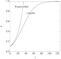
Fig. 2.16 from IPMB. A plot of the solution
of the logistic equation when y₀ = 0.1,
y_∞ = 1.0, b₀ = 0.0667. Exponential
growth with the same values of
y₀ and b₀ is also shown.

In Section 2.10 of Intermediate Physics for Medicine and Biology, Russ Hobbie and I discuss the logistic model.

Sometimes a growing population will level off at some constant value. Other times the population will grow and then crash. One model that exhibits leveling off is the logistic model, described by the differential equation

dy/dt = b₀ y (1 – y/y_∞) ,                           (2.28)

where b₀ and y_∞ are constants….

If the initial value of y is y₀, the solution of Eq. 2.28 is

y(t) = 1 / [1/y_∞ + (1/y₀ – 1/y_∞) e^−b₀t] .    (2.29)

Below is a new homework problem, analyzing the logistic equation in a way to build insight. Consider it an early Christmas present. Santa won’t give you the answer, so you need to solve the problem yourself to gain anything from this post.

Section 2.10

Problem 36 ½. Consider the logistic model.

(a) Write Eq. 2.28 in terms of dimensionless variables Y and T, where Y = y/y_∞ and T = b₀t.

(b) Express the solution Eq. 2.29 in terms of Y, T, and Y₀ = y₀/y_∞.

(c) Verify that your solution in part (b) obeys the differential equation you derive in part (a).

(d) Verify that your solution in part (b) is equal to Y₀ at T = 0.

(e) In a plot of Y(T) versus T, which of the three constants (y_∞, y₀, and b₀) affect the qualitative shape of the solution, and which just scale the Y and T axes? 

(f) Verify that your solution in part (b) approaches 1 as T goes to infinity.

(g) Find an expression for the slope of the curve Y = Y(T). What is the slope at time T = 0? For what value of Y₀ is the initial slope largest? For what values of Y₀ is the slope small?

(h) The plot in Fig. 2.16 compares the solution of logistic equation with the exponential Y = Y₀ e^T. The figure gives the impression that the exponential is a good approximation to the logistic curve at small times. Do the two curves have the same value at T = 0? Do the two curves have the same slope at T = 0?

(i) Sketch plots of Y versus T for Y₀ = 0.0001, 0.001, 0.01, and 0.1.

(j) Rewrite the solution from part (b), Y = Y(T), using the constant T₀, where T₀ = ln[(1−Y₀)/Y₀]. Show that varying Y₀ is equivalent to shifting the solution along the T axis. What value of Y₀ corresponds to T₀ = 0?

(k) How does the logistic curve behave if Y₀ > 1? Sketch a plot of Y versus T for Y₀ =1.5.

(l) How does the logistic curve behave if Y₀ < 0? Sketch a plot of Y versus T for Y₀ = –0.5.

(m) Plot Y versus T for Y₀ = 0.1 on semilog graph paper.

If you solve this new homework problem and want to compare you solution to mine, email me at roth@oakland.edu and I’ll send you my solution. 

The Logistic Equation, MIT OpenCourseWare

https://www.youtube.com/watch?v=TCkLSYxx21c&t=69s