Friday, October 28, 2016

dGEMRIC

dGEMRIC is an acronym for delayed gadolinium enhanced magnetic resonance imaging of cartilage. Adil Bashir and his colleagues provide a clear introduction to dGEMRIC in the abstract of their paper “Nondestructive Imaging of Human Cartilage Glycosaminoglycan Concentration by MRI” (Magnetic Resonance in Medicine, Volume 41, Pages 857–865, 1999).
Despite the compelling need mandated by the prevalence and morbidity of degenerative cartilage diseases, it is extremely difficult to study disease progression and therapeutic efficacy, either in vitro or in vivo (clinically). This is partly because no techniques have been available for nondestructively visualizing the distribution of functionally important macromolecules in living cartilage. Here we describe and validate a technique to image the glycosaminoglycan concentration ([GAG]) of human cartilage nondestructively by magnetic resonance imaging (MRI). The technique is based on the premise that the negatively charged contrast agent gadolinium diethylene triamine pentaacetic acid (Gd(DTPA)2-) will distribute in cartilage in inverse relation to the negatively charged GAG concentration. Nuclear magnetic resonance spectroscopy studies of cartilage explants demonstrated that there was an approximately linear relationship between T1 (in the presence of Gd(DTPA)2-) and [GAG] over a large range of [GAG]. Furthermore, there was a strong agreement between the [GAG] calculated from [Gd(DTPA)2-] and the actual [GAG] determined from the validated methods of calculations from [Na+] and the biochemical DMMB assay. Spatial distributions of GAG were easily observed in T1-weighted and T1-calculated MRI studies of intact human joints, with good histological correlation. Furthermore, in vivo clinical images of T1 in the presence of Gd(DTPA)2- (i.e., GAG distribution) correlated well with the validated ex vivo results after total knee replacement surgery, showing that it is feasible to monitor GAG distribution in vivo. This approach gives us the opportunity to image directly the concentration of GAG, a major and critically important macromolecule in human cartilage.
A schematic illustration of the structure of cartilage.
A schematic illustration of the
structure of cartilage.
The method is based on Donnan equilibrium, which Russ Hobbie and I describe in Section 9.1 of Intermediate Physics for Medicine and Biology. Assume the cartilage tissue (t) is bathed by saline (b). We will ignore all ions except the sodium cation, the chloride anion, and the negatively charged glycosaminoglycan (GAG). Cartilage is not enclosed by a semipermeable membrane, as analyzed in IPMB. Instead, the GAG molecules are fixed and immobile, so they act as if they cannot cross a membrane surrounding the tissue. Both the tissue and bath are electrically neutral, so [Na+]b = [Cl-]b and [Na+]t = [Cl-]t + [GAG-], where we assume GAG is singly charged (we could instead just interpret [GAG-] as being the fixed charge density). At the cartilage surface, sodium and chloride are distributed by a Boltzmann factor: [Na+]t/[Na+]b = [Cl-]b/[Cl-]t = exp(-eV/kT), where V is the electrical potential of the tissue relative to the bath, e is the elementary charge, k is the Boltzmann constant, and T is the absolute temperature. We can solve these equations for [GAG-] in terms of the sodium concentrations: [GAG-] = [Na+]b ( [Na+]t/[Na+]b - [Na+]b/[Na+]t ).

Now, suppose you add a small amount of gadolinium diethylene triamine pentaacetic acid (Gd-DTPA2-); so little that you can ignore it in the equations of neutrality above. The concentrations of Gd-DTPA on the two sides of the articular surface are related by the Boltzmann factor [Gd-DTPA2-]b/[Gd-DTPA2-]t = exp(-2eV/kT) [note the factor of two in the exponent reflecting the valance -2 of Gd-DTPA], implying that [Gd-DTPA2-]b/[Gd-DTPA2-]t = ( [Na+]t/[Na+]b )2. Therefore,

An equation giving the concentration of glycosaminoglycan in cartilage from the measured concentration of gadolinium diethylene triamine pentaacetic acid.

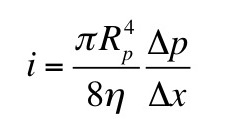
We can determine [GAG-] by measuring the sodium concentration in the bath and the Gd-DTPA concentration in the bath and the tissue. Section 18.6 of IPMB describes how gadolinium shortens the T1 time constant of a magnetic resonance signal, so using T1-weighted magnetic resonance imaging you can determine the gadolinium concentration in both the bath and the tissue.

From my perspective, I like dGEMRIC because it takes two seemingly disparate parts of IPMB, the section of Donnan equilibrium and the section on how relaxation times affect magnetic resonance imaging, and combines them to create an innovative imaging method. Bashir et al.’s paper is eloquent, so I will close this blog post with their own words.
The results of this study have demonstrated that human cartilage GAG concentration can be measured and quantified in vitro in normal and degenerated tissue using magnetic resonance spectroscopy in the presence of the ionic contrast agent Gd(DTPA)2- … These spectroscopic studies therefore demonstrate the quantitative correspondence between tissue T1 in the presence of Gd(DTPA)2- and [GAG] in human cartilage. Applying the same principle in an imaging mode to obtain T1 measured on a spatially localized basis (i.e., T1-calculated images), spatial variations in [GAG] were visualized and quantified in excised intact samples…

In summary, the data presented here demonstrate the validity of the method for imaging GAG concentration in human cartilage… We now have a unique opportunity to study developmental and degenerative disease processes in cartilage and monitor the efficacy of medical and surgical therapeutic measures, for ultimately achieving a greater understanding of cartilage physiology in health and disease.

Friday, October 21, 2016

The Nuts and Bolts of Life: Willem Kolff and the Invention of the Kidney Machine

The Nuts and Bolts of Life: Willem Kolff and the Invention of the Kidney Machine, by Paul Heiney, superimposed on Intermediate Physics for Medicine and BIology.
The Nuts and Bolts of Life:
Willem Kolff and the
Invention of the Kidney Machine,
by Paul Heiney.
In Chapter 5 of Intermediate Physics for Medicine and Biology, Russ Hobbie and I discuss the artificial kidney.
Two compartments, the body fluid and the dialysis fluid, are separated by a membrane that is porous to the small molecules to be removed and impermeable to larger molecules. If such a configuration is maintained long enough, then the concentration of any solute that can pass through the membrane will become the same on both sides.
The history of the artificial kidney is fascinating. Paul Heiney describes this story in his book The Nuts and Bolts of Life: Willem Kolff and the Invention of the Kidney Machine.
Willem Kolff…has battled to mend broken bodies by bringing mechanical solutions to medical problems. He built the first ever artificial kidney and a working artificial heart, and helped create the artificial eye. He s the true founder of the bionic age in which all human parts will be replaceable.
Heiney’s book is not a scholarly treatise and there is little physics in it, but Kolff’s personal story is captivating. Much of the work to develop the artificial kidney was done during World War II, when Kolff’s homeland, the Netherlands, was occupied by the Nazis. Kolff managed to create the first artificial organ while simultaneously caring for his patients, collaborating with the Dutch resistance, and raising five children. Kolff was a tinkerer in the best sense of the word, and his eccentric personality reminds me of the inventor of the implantable pacemaker, Wilson Greatbatch.

Below are some excepts from the first chapter of The Nuts and Bolts of Life. To learn more about Kolff, see his New York Times obituary.
What might a casual visitor have imagined was happening behind the closed door of Room 12a on the first floor of Kampen Hospital in a remote and rural corner of Holland on the night of 11 September 1945? There was little to suggest a small miracle was taking place; in fact, the sounds that emerged from that room could easily have been mistaken for an organized assault.

The sounds themselves were certainly sinister. There was a rumbling that echoed along the tiled corridors of the small hospital and kept patients on the floor below from their sleep; and the sound of what might be a paddle-steamer thrashing through water. All very curious…

The 67-year-old patient lying in Room 12a would have been oblivious to all this. During the previous week she had suffered high fever, jaundice, inflammation of the gall bladder and kidney failure. Not quite comatose, she could just about respond to shouts or the deliberative infliction of pain. Her skin was pale yellow and the tiny amount of urine she produced was dark brown and cloudy….

Before she was wheeled into Room 12a of Kampen Hospital that night, Sofia Schafstadt’s death was a foregone conclusion. There was no cure for her suffering; her kidneys were failing to cleanse her body of the waste it created in the chemical processes of keeping her alive. She was sinking into a body awash in her own poisons….

But that night was to be like no other night in medical history. The young doctor, Willem Kolff, then aged thirty-four and an internist at Kampen Hospital, brought to a great crescendo his work of much of the previous five years. That night, he connected Sofia Schafstadt to his artificial kidney – a machine born out of his own ingenuity. With it, he believed, for the first time ever he could replicate the function of one of the vital organs with a machine working outside the body…

The machine itself was the size of a sideboard and stood by the patient’s bed. The iron frame carried a large enamel tank containing fluid. Inside this rotated a drum around which was wrapped the unlikely sausage skin through which the patient’s blood flowed. And that, in essence, was it: a machine that could undoubtedly be called a contraption was about to become the world’s first successful artificial kidney…

Friday, October 14, 2016

John David Jackson (1925-2016)

Classical Electrodynamics, 3rd Ed, by John David Jackson, superimposed on Intermediate Physics for Medicine and Biology.
Classical Electrodynamics, 3rd Ed,
by John David Jackson.
John David Jackson died on May 20 of this year. I am familiar with Jackson mainly through his book Classical Electrodynamics. Russ Hobbie and I cite Jackson in Chapter 14 of Intermediate Physics for Medicine and Biology.
The classical analog of Compton scattering is Thomson scattering of an electromagnetic wave by a free electron. The electron experiences the electric field E of an incident plane electromagnetic wave and therefore has an acceleration −eE/m. Accelerated charges radiate electromagnetic waves, and the energy radiated in different directions can be calculated, giving Eqs. 15.17 and 15.19. (See, for example, Jackson 1999, Chap. 14.) In the classical limit of low photon energies and momenta, the energy of the recoil electron is negligible.
Classical Electrodynamics, 2nd Ed, by John David Jackson, superimposed on Intermediate Physics for Medicine and Biology.
Classical Electrodynamics, 2nd Ed,
by John David Jackson.
Classical Electrodynamics is usually known simply as “Jackson.” It is one of the top graduate textbooks in electricity and magnetism. When I was a graduate student at Vanderbilt University, I took an electricity and magnetism class based on the second edition of Jackson (the edition with the red cover). My copy of the 2nd edition is so worn that I have its spine held together by tape. Here at Oakland University I have taught from Jackson’s third edition (the blue cover). I remember my shock when I discovered Jackson had adopted SI units in the 3rd edition. He writes in the preface
My tardy adoption of the universally accepted SI system is a recognition that almost all undergraduate physics texts, as well as engineering books at all levels, employ SI units throughout. For many years Ed Purcell and I had a pact to support each other in the use of Gaussian units. Now I have betrayed him!
Classical Electrodynamics, by John David Jackson, editions 2 and 3, with Intermdiate Physics for Medicine and Biology.
Classical Electrodynamics,
by John David Jackson.
Jackson has been my primary reference when I need to solve problems in electricity and magnetism. For instance, I consider my calculation of the magnetic field of a single axon to be little more than a classic “Jackson problem.” Jackson is famous for solving complicated electricity and magnetism problems using the tools of mathematical physics. In Chapter 2 he uses the method of images to calculate the the force between a point charge q and a nearby conducting sphere having the same charge q distributed over its surface. When the distance between the charge and the sphere is large compared to the sphere radius, the repelling force is given by Coulombs law. When the distance is small, however, the charge induces a surface charge of opposite sign on the sphere near it, resulting in an attractive force. Later in Chapter 2, Jackson uses Fourier analysis to calculate the potential inside a two-dimension slot having a voltage V on the bottom surface and grounded on the sides. He finds a series solution, which I think I could have done myself, but then he springs an amazing trick with complex variables in order to sum the series and get an entirely nonintuitive analytical solution involving an inverse tangent of a sine divided by a hyperbolic sine. How lovely.

My favorite is Chapter 3, where Jackson solves Laplace’s equation in spherical and cylindrical coordinate systems. Nerve axons and strands of cardiac muscle are generally cylindrical, so I am a big user of his cylindrical solution based on Bessel functions and Fourier series. Many of my early papers were variations on the theme of solving Laplace’s equation in cylindrical coordinates. In Chapter 5, Jackson analyzes a spherical shell of ferromagnetic material, which is an excellent model for a magnetic shield used in biomagnetic studies.

I have spent most of my career applying what I learned in Jackson to problems in medicine and biology.

Friday, October 7, 2016

Data Reduction and Error Analysis for the Physical Sciences

Data Reduction and Error Analysis  for the Physical Sciences,  by Philip Bevington and Keith Robinson, superimposed on Intermediate Physics for Medicine and Biology.
Data Reduction and Error Analysis
for the Physical Sciences,
by Philip Bevington and Keith Robinson.
In Chapter 11 of Intermediate Physics for Medicine and Biology, Russ Hobbie and I cite the book Data Reduction and Error Analysis for the Physical Sciences, by Philip Bevington and Keith Robinson.
The problem [of fitting a function to data] can be solved using the technique of nonlinear least squares…The most common [algorithm] is called the Levenberg-Marquardt method (see Bevington and Robinson 2003 or Press et al. 1992).
I have written about the excellent book Numerical Recipes by Press et al. previously in this blog. I was not too familiar with the book by Bevington and Robinson, so last week I checked out a copy from the Oakland University library (the second edition, 1992).

I like it. The book is a great resource for many of the topics Russ and I discuss in IPMB. I am not an experimentalist, but I did experiments in graduate school, and I have great respect for the challenges faced when working in the laboratory.

Their Chapter 1 begins by distinguishing between systematic and random errors. Bevington and Robinson illustrate the difference between accuracy and precision using a figure like this one:

An illustration showing the difference between precise but inaccurate data ad accurate but imprecise data.
a) Precise but inaccurate data. b) Accurate but imprecise data.

Next, they present a common sense discussion about significant figures, a topic that my students often don’t understand. (I assign them a homework problem with all the input data to two significant figures, and they turn in an answer--mindlessly copied from their calculator--containing 12 significant figures.)

In Chapter 2 of Data Reduction and Error Analysis, Bevington and Robinson introduce probability distributions.
Of the many probability distributions that are involved in the analysis of experimental data, three play a fundamental role: the binomial distribution [Appendix H in IPMB], the Poisson distribution [Appendix J], and the Gaussian distribution [Appendix I]. Of these, the Gaussian or normal error distribution is undoubtedly the most important in statistical analysis of data. Practically, it is useful because it seems to describe the distribution of random observations for many experiments, as well as describing the distributions obtained when we try to estimate the parameters of most other probability distributions.
Here is something I didn’t realize about the Poisson distribution:
The Poisson distribution, like the bidomial distribution, is a discrete distribution. That is, it is defined only at integral values of the variable x, although the parameter μ [the mean] is a positive, real number.
Figure J.1 of IPMB plots the Poisson distribution P(x) as a continuous function. I guess the plot should have been a histogram.

Chapter 3 addresses error analysis and propagation of error. Suppose you measure two quantities, x and y, each with an associated standard deviation σx and σy. Then you calculate a third quantity z(x,y). If x and y are uncorrelated, then the error propagation equation is
An equation for the propagation of error.
For instance, Eq. 1.40 in IPMB gives the flow of a fluid through a pipe, i, as a function of the viscosity of the fluid, η, and the radius of the pipe, Rp
An equation for flow through a pipe.
The error propagation equation (and some algebra) gives the standard deviation of the flow in terms of the standard deviation of the viscosity and the standard deviation of the radius
When you have a variable raised to the fourth power, such as the pipe radius in the equation for flow, it contributes four times more to the flow’s percentage uncertainty than a variable such as the viscosity. A ten percent uncertainty in the radius contributes a forty percent uncertainty to the flow. This is a crucial concept to remember when performing experiments.

Bevington and Robinson derive the method of least squares in Chapter 4, covering much of the same ground as in Chapter 11 of IPMB. I particularly like the section titled A Warning About Statistics.
Equation (4.12) [relating the standard deviation of the mean to the standard deviation and the number of trails] might suggest that the error in the mean of a set of measurements xi can be reduced indefinitely by repeated measurements of xi. We should be aware of the limitations of this equation before assuming that an experimental result can be improved to any desired degree of accuracy if we are willing to do enough work. There are three main limitations to consider, those of available time and resources, those imposed by systematic errors, and those imposed by nonstatistical fluctuations.
Russ and I mention Monte Carlo techniques—the topic of Chapter 5 in Data Reduction and Error Analysis—a couple times in IPMB. Then Bevington and Robinson show how to use least squares to fit to various functions: a line (Chapter 6), a polynomial (Chapter 7), and an arbitrary function (Chapter 8). In Chapter 8 the Marquardt method is introduced. Deriving this algorithm is too involved for this blog post, but Bevington and Robinson explain all the gory details. They also provide much insight about the method, such as in the section Comments on the Fits:
Although the Marquardt method is the most complex of the four fitting routines, it is also the clear winner for finding fits most directly and efficiently. It has the strong advantage of being reasonably insensitive of the starting values of the parameters, although in the peak-over-background example in Chapter 9, it does have difficulty when the starting parameters of the function for the peak are outside reasonable ranges. The Marquardt method also has the advantage over the grid- and gradient-search methods of providing an estimate of the full error matrix and better calculation of the diagonal errors.
The rest of the book covers more technical issues that are not particularly relevant to IPMB. The appendix contains several computer programs written in Pascal. The OU library copy also contains a 5 1/2 inch floppy disk, which would have been useful 25 years ago but now is quaint.

Philip Bevington wrote the first edition of Data Reduction and Error Analysis in 1969, and it has become a classic. For many years he was a professor of physics at Case Western University, and died in 1980 at the young age of 47. A third edition was published in 2002. Download it here.