 |
| Data Reduction and Error Analysis for the Physical Sciences, by Philip Bevington and Keith Robinson. |
The problem [of fitting a function to data] can be solved using the technique of nonlinear least squares…The most common [algorithm] is called the Levenberg-Marquardt method (see Bevington and Robinson 2003 or Press et al. 1992).I have written about the excellent book Numerical Recipes by Press et al. previously in this blog. I was not too familiar with the book by Bevington and Robinson, so last week I checked out a copy from the Oakland University library (the second edition, 1992).
I like it. The book is a great resource for many of the topics Russ and I discuss in IPMB. I am not an experimentalist, but I did experiments in graduate school, and I have great respect for the challenges faced when working in the laboratory.
Their Chapter 1 begins by distinguishing between systematic and random errors. Bevington and Robinson illustrate the difference between accuracy and precision using a figure like this one:
 |
a) Precise but inaccurate data. b) Accurate but imprecise data.
|
In Chapter 2 of Data Reduction and Error Analysis, Bevington and Robinson introduce probability distributions.
Of the many probability distributions that are involved in the analysis of experimental data, three play a fundamental role: the binomial distribution [Appendix H in IPMB], the Poisson distribution [Appendix J], and the Gaussian distribution [Appendix I]. Of these, the Gaussian or normal error distribution is undoubtedly the most important in statistical analysis of data. Practically, it is useful because it seems to describe the distribution of random observations for many experiments, as well as describing the distributions obtained when we try to estimate the parameters of most other probability distributions.Here is something I didn’t realize about the Poisson distribution:
The Poisson distribution, like the bidomial distribution, is a discrete distribution. That is, it is defined only at integral values of the variable x, although the parameter μ [the mean] is a positive, real number.Figure J.1 of IPMB plots the Poisson distribution P(x) as a continuous function. I guess the plot should have been a histogram.
Chapter 3 addresses error analysis and propagation of error. Suppose you measure two quantities, x and y, each with an associated standard deviation σx and σy. Then you calculate a third quantity z(x,y). If x and y are uncorrelated, then the error propagation equation is
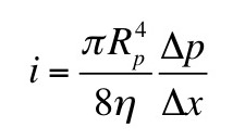
For instance, Eq. 1.40 in IPMB gives the flow of a fluid through a pipe, i, as a function of the viscosity of the fluid, η, and the radius of the pipe, Rp
When you have a variable raised to the fourth power, such as the pipe radius in the equation for flow, it contributes four times more to the flow’s percentage uncertainty than a variable such as the viscosity. A ten percent uncertainty in the radius contributes a forty percent uncertainty to the flow. This is a crucial concept to remember when performing experiments.
Bevington and Robinson derive the method of least squares in Chapter 4, covering much of the same ground as in Chapter 11 of IPMB. I particularly like the section titled A Warning About Statistics.
Equation (4.12) [relating the standard deviation of the mean to the standard deviation and the number of trails] might suggest that the error in the mean of a set of measurements xi can be reduced indefinitely by repeated measurements of xi. We should be aware of the limitations of this equation before assuming that an experimental result can be improved to any desired degree of accuracy if we are willing to do enough work. There are three main limitations to consider, those of available time and resources, those imposed by systematic errors, and those imposed by nonstatistical fluctuations.Russ and I mention Monte Carlo techniques—the topic of Chapter 5 in Data Reduction and Error Analysis—a couple times in IPMB. Then Bevington and Robinson show how to use least squares to fit to various functions: a line (Chapter 6), a polynomial (Chapter 7), and an arbitrary function (Chapter 8). In Chapter 8 the Marquardt method is introduced. Deriving this algorithm is too involved for this blog post, but Bevington and Robinson explain all the gory details. They also provide much insight about the method, such as in the section Comments on the Fits:
Although the Marquardt method is the most complex of the four fitting routines, it is also the clear winner for finding fits most directly and efficiently. It has the strong advantage of being reasonably insensitive of the starting values of the parameters, although in the peak-over-background example in Chapter 9, it does have difficulty when the starting parameters of the function for the peak are outside reasonable ranges. The Marquardt method also has the advantage over the grid- and gradient-search methods of providing an estimate of the full error matrix and better calculation of the diagonal errors.The rest of the book covers more technical issues that are not particularly relevant to IPMB. The appendix contains several computer programs written in Pascal. The OU library copy also contains a 5 1/2 inch floppy disk, which would have been useful 25 years ago but now is quaint.
Philip Bevington wrote the first edition of Data Reduction and Error Analysis in 1969, and it has become a classic. For many years he was a professor of physics at Case Western University, and died in 1980 at the young age of 47. A third edition was published in 2002. Download it here.


Russ just pointed out that Fig. J.1 is NOT a plot of P(x). It plots P versus m=NDeltat, which can vary continuously. "I thought I was wrong once, but I was mistaken."
ReplyDelete