More about the Stopping Power and the Bragg Peak

The Bragg peak is a key concept when studying the interaction of protons with tissue. In Chapter 16 of the 4th edition of Intermediate Physics for Medicine and Biology, Russ Hobbie and I write

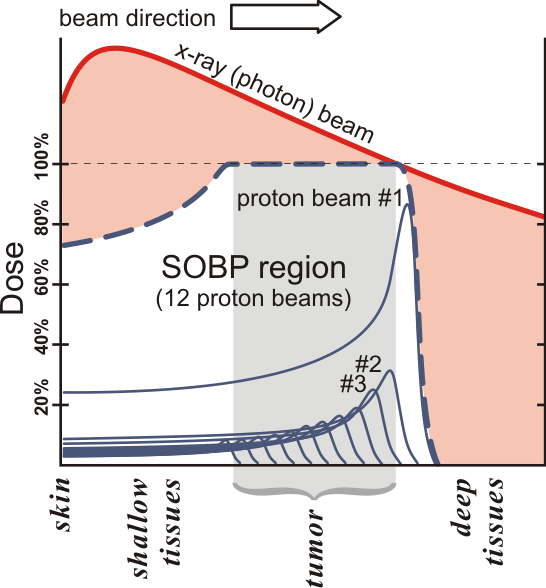
Protons are also used to treat tumors. Their advantage is the increase of stopping power at low energies. It is possible to make them come to rest in the tissue to be destroyed, with an enhanced dose relative to intervening tissue and almost no dose distally (“downstream”) as shown by the Bragg peak in Fig. 16.51 [see a similar figure here]. Placing an absorber in the proton beam before it strikes the patient moves the Bragg peak closer to the surface. Various techniques, such as rotating a variable-thickness absorber in the beam, are used to shape the field by spreading out the Bragg peak (Fig. 16.52) [see a similar figure here].

Figure 16.52 is very interesting, because it shows a nearly uniform dose throughout a region of tissue produced by a collection of Bragg peaks, each reaching a maximum at a different depth because the protons have different initial energies. The obvious question is: how many protons should one use for each energy to produce a uniform dose in some region of tissue? I have discussed the Bragg peak before in this blog, when I presented a new homework problem to derive an analytical expression for the stopping power as a function of depth. An extension of this problem can be used to answer this question. Russ and I considered including this extended problem in the 5th edition of IPMB (which is nearing completion), but it didn’t make the cut. Discarded scraps from the cutting room floor make good blog material, so I present you, dear reader, with a new homework problem.

Problem 31 3/4 A proton of kinetic energy T is incident on the tissue surface (x = 0). Assume its stopping power s(x) at depth x is given by

where C is a constant characteristic of the tissue.

(a) Plot s(x) versus x. Where does the Bragg peak occur?

(b) Now, suppose you have a distribution of N protons. Let the number with incident energy between T and T+dT be A(T)dT, where

Determine the constant B by requiring

Plot A(T) vs T.

(c) If x is greater than T₂²/2C what is the total stopping power? Hint: think before you calculate; how many particles can reach a depth greater than T₂²/2C?

(d) If x is between T₁²/2C and T₂²/2C, only particles with energy from (2Cx)^1/2 to T₂ contribute to the stopping power at x, so

Evaluate this integral. Hint: let u = T² - (2Cx + T₂²)/2.

(e) If x is less than T₁²/2C, all the particles contribute to the stopping power at x, so

Evaluate this integral.

(f) Plot S(x) versus x. Compare your plot with that found in part a, and with Fig. 16.52.

One reason this problem didn’t make the cut is that it is rather difficult. Let me know if you need the solution. The bottom line: this homework problem does a pretty good job of explaining the results in Fig. 16.52, and provides insight into how to apply proton therapy to an large tumor.