Friday, July 7, 2023

Integral of the Bessel Function

Have you ever been reading a book, making good progress with everything making sense, and then you suddenly stop at say “wait… what?”. That happened to me recently as I was reading Homework Problem 31 in Chapter 12 of Intermediate Physics for Medicine and Biology. (Wait…what? I’m a coauthor of IPMB! How could there be any surprises for me?) The problem is about calculating the two-dimensional Fourier transform of 1/r, and it supplies the following Bessel function identity 

An equation for the integral of the Bessel function J0(kr).

The function J0 is a Bessel function of the first kind of order zero. What surprised me is that if you let x = kr, you get that the integral of the Bessel function is one,

An equation for the integral of the Bessel function J0(x), which equals one.

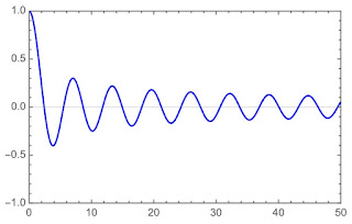
Really? Here’s a plot of J0(x).

A plot of the J0(x) Bessel function versus x.

It oscillates like crazy and the envelope of those oscillations falls off very slowly. In fact, an asymptotic expansion for J0 at large x is

An asymptotic expression for the J0 Bessel function at large argument.

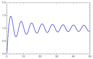
The leading factor of 1/√x decays so slowly that its integral from zero to infinity does not converge. Yet, when you include the cosine so the function oscillates, the integral does converge. Here’s a plot of

An expression for the integral of the Bessel function J0(x') from 0 to x.

A plot of the integral of the J0 Bessel function.

The integral approaches one at large x, but very slowly. So, the expression given in the problem is correct, but I sure wouldn’t want to do any numerical calculations using it, where I had to truncate the endpoint of the integral to something less than infinity. That would be a mess!

Here’s another interesting fact. Bessel functions come in many orders—J0, J1, J2, etc.—and they all integrate to one.

Who’s responsible for these strangely-behaved functions? They’re named after the German astronomer Friedrich Bessel but they were first defined by the Swiss mathematician Daniel Bernoulli (1700–1782), a member of the brilliant Bernoulli family. The Bernoulli equation, mentioned in Chapter 1 of IPMB, is also named for Daniel Bernoulli. 

There was a time when I was in graduate school that I was obsessed with Bessel functions, especially modified Bessel functions that don’t oscillate. I’m not so preoccupied by them now, but they remain my favorite of the many special functions encountered in physics.

Friday, June 30, 2023

Gauss and von Humboldt

The Age of Napoleon,
by Will and Ariel Durant,
Volume 11 of The Story of Civilization.


Regular readers of this blog may recall that over the last few years I’ve been reading Will and Ariel Durant’s magnificent The Story of Civilization. I’m almost done.  I’m currently finishing the final chapters of the last volume: The Age of Napoleon. In the chapter about the German people is a section on science. It states
Two men especially brought scientific honors to Germany in this age—Karl Friedrich Gauss (1777–1855) and Alexander von Humboldt (1769–1859).
Humboldt is never mentioned in Intermediate Physics for Medicine and Biology, but Gauss is everywhere. When speaking of Gauss, the Durants write
We shall not pretend to understand, much less to expound, the discoveries—in number theory, imaginary numbers, quadratic residues, the method of least squares, the infinitesimal calculus—by which Gauss transformed mathematics from what it had been in Newton’s time into an almost new science, which became a tool of the scientific miracles of our time. His observations of the orbit of Ceres (the first planetoid, discovered on January 1, 1801) led him to formulate a new and expeditious method of determining planetary orbits [least squares is discussed in Chapter 11 of IPMB]. He made researches which placed the theory of magnetism and electricity upon a mathematical basis [Gauss’s law for calculating the electric field is discussed in Chapter 6 of IPMB; the now somewhat obsolete unit of magnetic field strength is the gauss]. He was a burden and blessing [definitely a blessing] to all scientists, who believe that nothing is science until it can be stated in mathematical terms. [He also invented the Gaussian probability distribution, which plays a major role in diffusion, discussed in Chapter 4 of IPMB]…. He is now ranked with Archimedes and Newton.
Humboldt was more of a naturalist, and his name never appears in IPMB. But the Durants devoted even more space in their history to him than to Gauss.
The other hero of German Science in this age was Wilhelm von Humboldt’s younger brother Alexander…. In 1796 he began, by accident, the long tour of scientific discovery (rivaling Darwin’s on the Beagle) whose results made him, according to a contemporary quip, “the most famous man in Europe, next to Napoleon.”
Humboldt is particularly famous for his work in geography and geology. I become familiar with him when I taught earth science. I was a new, untenured faculty member at Oakland University when the physics department needed someone to teach our earth science class. OU does not have a geology department, but some students do need a course in earth science, so the physics department was in charge of it. When the faculty member who traditionally taught it retired, I was asked to take it over. I knew nothing about earth science, but neither did anyone else in the department, and being the newest member of the department I didn’t feel that I could say no. I taught the class for about five years, and found that I enjoyed it. Most students in the course were elementary education majors. They weren’t the strongest science students I ever taught, but they were some of the nicest.

Here is what the Durants had to say about Humboldt.
He discovered (1804) that the earth’s magnetic force decreases in intensity from the poles to the equator. He enriched geology with his studies of the igneous origin of certain rocks, the formation of mountains, the geographical distribution of volcanoes. He provided the earliest clues to the laws governing atmospheric disturbances, and thereby shed light on the origin and direction of tropical storms. He made classic studies of air and ocean currents…. His Essai sur la geographie des plantes began the science of biogeography—the study of plant distribution as affected by the physical conditions of the terrain. These and a hundred other contributions, modest in appearance but of wide and lasting influence, were published in thirty volumes from 1805 to 1834 as Voyages de Humboldt et Bonpland aux regions equinoxiales du nouveau continent.

Humboldt is particularly relevant these days as one of the first environmentalists and discoverer of the concept of human-induced climate change. The closest he came to IPMB may be his work on muscle excitation and bioelectricity. In “Alexander von Humboldt and the Concept of Animal Electricity” (Trends in Neurosciences, Volume 20, Pages 239–242, 1997), Helmut Kettenmann wrote

More than two hundred years ago, Alexander von Humboldt helped to establish Galvani's view that muscle and nerve tissue are electrically excitable. His 1797 publication was a landmark for establishing the concept of animal electricity. Almost half a century later, von Humboldt became the mentor of the young du Bois-Reymond. With the help of von Humboldt's promotion, du Bois-Reymond demonstrated convincingly that animal tissue has the intrinsic capacity to generate electrical activity, and thus laid the ground for modern electrophysiology

Gauss and Humboldt; what a pair. Put them together with Goethe and Beethoven and Germany around 1800 becomes a pretty interesting place.

Oh, what will I do with myself now that my reading of The Story of Civilization is complete? I guess I will have to focus on the 6th edition of IPMB.


My favorite Gauss story, about how as a child he added all the numbers from 1 to 100.

https://www.youtube.com/watch?v=cD9rI4wSc7o

Ken Jennings narrates this video about Alexander von Humboldt.

https://www.youtube.com/watch?v=fj7tRMdmOgs

Alexander von Humboldt and the discovery of climate change.

https://www.youtube.com/watch?v=fYrXE_umWCw

Friday, June 23, 2023

The Partition Function

Any good undergrad statistical mechanics class analyzes the partition function. However, Russ Hobbie and I don’t introduce the partition function in Intermediate Physics for Medicine and Biology. Why not? Its a long story.

Russ and I do discuss the Boltzmann factor. Suppose you have a system that is in thermal equilibrium with a reservoir at absolute temperature T. Furthermore, suppose your system has discrete energy levels with energy Ei, where i is just an integer labeling the levels. The probability Pi of the system being in level i, is proportional to the Boltzmann factor, exp(–Ei/kBT),

Pi = C exp(–Ei/kBT),

where exp is the exponential function, kB is the Boltzmann constant and C is a constant of proportionality. How do you find C? Any probability must be normalized: the sum of the probabilities must equal one,

Σ Pi = 1 ,

where Σ indicates a summation over all values of i. This means

Σ C exp(–Ei/kBT) = 1,

or

C = 1/[Σ exp(–Ei/kBT)] .

The sum in the denominator is the partition function, and is usually given the symbol Z,

Z = Σ exp(–Ei/kBT) .

In terms of the partition function, the probability of being in state Pi is simply

Pi = (1/Z) exp(–Ei/kBT) .

An Introduction to Thermal Physics, superimposed on Intermediate Physics for Medicine and Biology.
An Introduction to Thermal Physics,
by Daniel Schroeder.
Here is what Daniel Schroeder writes in his excellent textbook An Introduction to Thermal Physics,
The quantity Z is called the partition function, and turns out to be far more useful than I would have suspected. It is a “constant” in that it does not depend on any particular state s [he uses “s” rather than “i” to count states], but it does depend on temperature. To interpret it further, suppose once again that the ground state has energy zero. Then the Boltzmann factor for the ground state is 1, and the rest of the Boltzmann factors are less than 1, by a little or a lot, in proportion to the probabilities of the associated states. Thus, the partition function essentially counts how many states are accessible to the system, weighting each one in proportion to its probability.
To see why it’s so useful, let’s define β as 1/kBT. The Boltzmann factor is then

exp(–βEi)

and the partition function is

Z = Σ exp(–βEi) .

The average energy, <E>, is

<E> =
Ei exp(–βEi)]/[Σ exp(–βEi)] .

The denominator is just Z. The numerator can be written as the negative of the derivative of Z with respect to
β, dZ/dβ (try it and see). So, the average energy is

<E> = – (1/Z)
dZ/dβ .

I won’t go on, but there are other quantities that are similarly related to the partition function. It
s surprisingly useful.

Is the partition function hidden in IPMB? You might recognize it in Eq. 3.37, which determines the average kinetic energy of a particle at temperature T (the equipartition of energy theorem) It looks a little different, because there
s a continuous range of energy levels, so the sum is disguised as an integral. You can see it again in Eq. 18.8, when evaluating the average value of the magnetic moment during magnetic resonance imaging. The partition functions there, but its nameless.

Why didn
t Russ and I introduce the partition function? In the Introduction of IPMB Russ wrote: “Each subject is approached in as simple a fashion as possible. I feel that sophisticated mathematics, such as vector analysis or complex exponential notation, often hides physical reality from the student.” Like Russ, I think that the partition function is a trick that makes some equations more compact, but hides the essential physics. So we didnt use it.

Friday, June 16, 2023

LaTeX and Mathematica

The front cover of Intermediate Physics for Medicine and Biology.
Gene Surdutovich and I are hard at work on the 6th edition of Intermediate Physics for Medicine and Biology. So far, the main thrust of our work involves LaTeX and Mathematica.

Russ Hobbie and I wrote the 5th edition of IPMB using LaTeX, a computer program that is particularly useful for typesetting equations. Russ was our LaTeX guru. I merely read pdf documents that he created and sent him my suggested changes, and then he implemented those changes into the book. With Russ gone, I can no longer escape dealing with LaTeX commands. LaTeX is an extremely powerful piece of software, but mastering it requires a long learning curve. Fortunately, Gene has extensive experience with it.

Let me give you a little peek behind the curtain at typesetting an equation with LaTeX. Equation 4.74 in the 5th edition is the definition of the error function,

In LaTeX it looks like this:

\begin{equation}
\operatorname{erf}(z)=\frac{2}{\sqrt{\uppi}}\int_{0}^{z}e^{-t^{2}}dt.
\label{4.74}%
\end{equation}

Kind of complicated, isn’t it? Sometimes I find myself getting LaTeX and html mixed up. 

LaTeX numbers the equations automatically. They each get a label, such as “\label{4.74}” but this label does not specify the equation number, it’s just a pointer. If I want to refer to this equation later I can write “see Eq.~\ref{4.74}”. If I decide I want to add an equation before Eq. 4.74, I can just give it any label I want—say, “\label{4.73b}”— and then LaTeX will renumber all the equations properly. For a book like IPMB, which has hundreds of equations, this automatic numbering is wonderful.

The index is also created automatically. Whenever I use a term such as “error function” that I want included in the index, I add “\index{Error function}”. LaTeX will keep track of the page number where that code is placed and then include that term with the correct page number in the index. This same sort of internal labeling can be used to create the list of symbols at the end of each chapter,  the list of homework problems, and the section and subsection numbering. In fact, I didn’t have to renumber anything when I added an entire new chapter about... more on that later. LaTeX is amazing. How did I write my PhD dissertation without it?

Also, LaTeX can number and label figures and illustrations, but you have to create the figures using another program. We’ve started using Mathematica for that job. (I’m ashamed to say, I’m not sure what software Russ used.) Mathematica, produced by Wolfram Research, is very powerful, and can do all sorts of symbolic computations. We don’t take advantage of those features, but mainly use the program to make beautiful plots. Fortunately, Gene is even better at Mathematica than at LaTeX, and he helps me a lot. IPMB’s publisher, Springer, says we can use as much color as we want for the 6th edition. Think of the 5th edition of IPMB as like when Dorothy is in Kansas. Publication of the 6th edition will correspond to that memorable scene when she opens the door of the farmhouse and finds herself in the colorful Land of Oz.

Preparing the 6th edition is going to be a long-term project, so don’t expect it anytime soon. Maybe it’ll be ready by the end of 2024, but maybe not. Thanks to all of you who responded to our recent survey. If you have further suggestions, there is still lots of time and we would appreciate hearing any ideas.

And now, back to work!

Dorothy enters the Land of Oz.

https://www.youtube.com/watch?v=F4eQmTizTSo


“If I Only Had a Brain”, from the Wizard of Oz. The song has nothing to do with LaTeX or Mathematica or IPMB, but it’s such a great number that you just have to watch.

https://www.youtube.com/watch?v=nauLgZISozs


Friday, June 9, 2023

Is Quantum Mechanics Necessary for Understanding Magnetic Resonance?

Is Quantum Mechanics Necessary for Understanding Magnetic Resonance? superimposed on Intermediate Physics for Medicine and Biology.
Hanson, L.,
Is Quantum Mechanics Necessary for
Understanding Magnetic Resonance?

Concepts Magn.Reson., 32:329–340, 2008
In Chapter 18 of Intermediate Physics for Medicine and Biology, Russ Hobbie and I discuss magnetic resonance imaging. Like many authors, we derive an expression for the magnetization of the tissue using quantum mechanics. Must we use quantum theory? In an article published in Concepts in Magnetic Resonance, Lars Hanson asks the same question: “Is Quantum Mechanics Necessary for Understanding Magnetic Resonance?” (Volume 32, Pages 329–340, 2008). The abstract is given below.
Educational material introducing magnetic resonance typically contains sections on the underlying principles. Unfortunately the explanations given are often unnecessarily complicated or even wrong. Magnetic resonance is often presented as a phenomenon that necessitates a quantum mechanical explanation whereas it really is a classical effect, i.e. a consequence of the common sense expressed in classical mechanics. This insight is not new, but there have been few attempts to challenge common misleading explanations, so authors and educators are inadvertently keeping myths alive. As a result, new students’ first encounters with magnetic resonance are often obscured by explanations that make the subject difficult to understand. Typical problems are addressed and alternative intuitive explanations are provided.
How would IPMB have to be changed to remove quantum mechanics from the analysis of MRI? Quantum ideas first appear in the last paragraph of Section 18.2 about the source of the magnetic moment, where we introduce the idea that the z-component of the nuclear spin in a magnetic field is quantized and can take on values that are integral multiples of the reduced Planck’s constant, ℏ. Delete that paragraph.

Section 18.3 is entirely based on quantum mechanics. To find the average value of the z-component of the spin, we sum over all quantum states, weighted by the Boltzmann factor. The end result is an expression for the magnetization as a function of the magnetic field. We could, alternatively, do this calculation classically. Below is a revised Section 18.3 that uses only classical mechanics and classical thermodynamics.
18.3 The Magnetization

The MR [magnetic resonance] image depends on the magnetization of the tissue. The magnetization of a sample, M, is the average magnetic moment per unit volume. In the absence of an external magnetic field to align the nuclear spins, the magnetization is zero. As an external magnetic field B is applied, the spins tend to align in spite of their thermal motion, and the magnetization increases, proportional at first to the external field. If the external field is strong enough, all of the nuclear magnetic moments are aligned, and the magnetization reaches its saturation value.

We can calculate how the magnetization depends on B. Consider a collection of spins of a nuclear species in an external magnetic field. This might be the hydrogen nuclei (protons) in a sample. The spins do not interact with each other but are in thermal equilibrium with the surroundings, which are at temperature T. We do not consider the mechanism by which they reach thermal equilibrium. Since the magnetization is the average magnetic moment per unit volume, it is the number of spins per unit volume, N, times the average magnetic moment of each spin: M=N<μ>, where μ is the magnetic moment of a single spin.

To obtain the average value of the z component of the magnetic moment, we must average over all spin directions, weighted by the probability that the z component of the magnetic moment is in that direction. Since the spins are in thermal equilibrium with the surroundings, the probability is proportional to the Boltzmann factor of Chap. 3, e–(U/kBT) = eμBcosθ/kBT, where kB is the Boltzmann constant. The denominator in Eq. 18.8 normalizes the probability:


The factor of sinθ arises when calculating the solid angle in spherical coordinates (see Appendix L). At room temperature μB/(kBT) ≪ 1 (see Problem 4), and it is possible to make the approximation ex ≈ 1 + x. The integral in the numerator then has two terms:
The first integral vanishes. The second is equal to 2/3 (hint: use the substitution u = cosθ). The denominator is

The first integral is 2; the second vanishes. Therefore we obtain
The z component of M is


which is proportional to the applied field.
The last place quantum mechanics is mentioned is in Section 18.6 about relaxation times. The second paragraph, starting “One way to analyze the effect…”, can be deleted with little loss of meaning; it is almost an aside.

So, to summarize, if you want to modify Chapter 18 of IPMB to eliminate any reference to quantum mechanics, then 1) delete the last paragraph of Section 18.2, 2) replace Section 18.3 with the modified text given above, and 3) delete the second paragraph in Section 18.6. Then, no quantum mechanics appears, and Planck’s constant is absent. Everything is classical, just the way I like it.

Friday, June 2, 2023

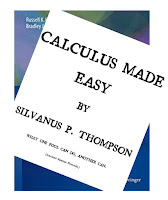
Calculus Made Easy

Intermediate Physics for Medicine and Biology assumes the reader knows calculus. Most medical doctors and biologists have studied some calculus, but I’m not sure they remember much of it. And most high school students, and even college freshman, have yet to take their first calculus course. What should these readers of IPMB do if they don’t know any calculus?  

Calculus Made Easy,
by Silvanus Thompson.
What these readers need is a quick and easy way to learn calculus without delving into all the subtle and complicated details. How can they do that? Read the delightful old book Calculus Made Easy, by Silvanus Thompson. Here’s the prologue:

Considering how many fools can calculate, it is surprising that it should be thought either a difficult or a tedious task for any other fool to learn how to master the same tricks. 
Some calculus-tricks are quite easy. Some are enormously difficult. The fools who write the textbooks of advanced mathematics — and they are mostly clever fools — seldom take the trouble to show you how easy the easy calculations are. On the contrary, they seem to desire to impress you with their tremendous cleverness by going about it in the most difficult way. 
Being myself a remarkably stupid fellow, I have had to unteach myself the difficulties, and now beg to present to my fellow fools the parts that are not hard. Master these thoroughly, and the rest will follow. What one fool can do, another can.
I know what you’re thinking: “That sounds like just what I need, but how much is it going to cost me?” The good news is that you can access the book for free online, at http://calculusmadeeasy.org.
Silvanus P. Thompson

The author, Silvanus Phillips Thompson (1851–1916), was an English physicist and a fellow of the Royal Society. I have a particular fondness for physicists from the Victorian era, especially one such as Thompson who was interested in science education and whose strength was his ability to explain difficult concepts clearly.

For those of you turned off by the dated style of Calculus Made Easy, written in 1910, I suggest Quick Calculus or Used Math instead. For those who, like me, love the Victorian style, I recommend Flatland by Edwin Abbott.

Enjoy!

Calculus Made Easy, by Silvanus P. Thompson, Part 1/2. A LibriVox audiobook. 

https://www.youtube.com/watch?v=hF2FLi5UnlE


Calculus Made Easy, by Silvanus P. Thompson, Part 2/2. A LibriVox audiobook.

https://www.youtube.com/watch?v=uqQtQNTKo-A

Friday, May 26, 2023

Terminal Speed of Microorganisms

A Paramecium aurelia seen through an optical microscope
A Paramecium aurelia seen through an optical microscope.
Source: Wikipedia (http://en.wikipedia.org/wiki/Image:Paramecium.jpg)

Homework Problem 28 at the end of Chapter 2 in Intermediate Physics for Medicine and Biology asks the reader to calculate the terminal speed of an animal falling in air. Although this problem provides insight, it includes a questionable assumption. Russ and I tell the student to “assume that the frictional force is proportional to the surface area of the animal.” If, however, the animal falls at low Reynolds number, this assumption is not valid. Instead, the drag force is given by Stokes’ law, which is proportional to the radius, not the surface area (radius squared). The new homework problem given below asks the reader to calculate the terminal speed for a microorganism falling through water at low Reynolds number.

Section 2.8

Problem 28 ½. Calculate the terminal speed, V, of a paramecium sinking in water. Assume that the organism is spherical with radius R, and that the Reynolds number is small so that the drag force is given by Stokes’ law. Include the effect of buoyancy. Let the paramecium’s radius be 100 microns and its specific gravity be 1.05. Verify that its Reynolds number is small.
The reader will first need to get the density ρ and viscosity η of water, which are ρ = 1000 kg/m3 and η = 0.001 kg/(m s). The specific gravity is not defined in IPMB, but it’s the density divided by the density of water, implying that the density of the paramecium is 1050 kg/m3. Finally, Stokes’ law is given in IPMB as Eq. 4.17, Fdrag = –6πRηV.

I’ll let you do your own calculation. I calculate the terminal speed to be about 1 mm/s, so it takes about a fifth of a second to sink one body diameter. The Reynolds number is 0.1, which is small, but not exceptionally small.

You should find that the terminal speed increases as the radius squared, in contrast to a drag force proportional to the surface area for which the terminal speed increases in proportion to the radius. Bigger organisms sink faster. The dependence of terminal speed on size is even more dramatic for aquatic microorganisms than for mammals falling in air. To paraphrase Haldane’s quip, “a bacterium is killed, a diatom is broken, a paramecium splashes,” except the speeds are small enough that none of the “wee little beasties” are really killed (the terminal speed is not terminal...get it?) and splashing is a high Reynolds number phenomenon.

Buoyancy is not negligible for aquatic animals. The effective density of a paramecium in air would be about 1000 kg/m3, but in water its effective density drops to a mere 50 kg/m3. Microorganisms are made mostly of water, so they are almost neutrally buoyant. In this homework problem, the effect of gravity is reduced to only five percent of what it would be if buoyancy were ignored.

A paramecium is a good enough swimmer that it can swim upward against gravity if it wants to. Its surface is covered with cilia that beat together like a Roman galley to produce the swimming motion (ramming speed!).

Whenever discussing terminal speed, one should remember that we assume the fluid is initially at rest. In fact, almost any volume of water will have currents moving at speeds greater than 1 mm/s, caused by tides, gravity, thermal convection, wind driven waves, or the wake of a fish swimming by. A paramecium would drift along with these currents. To observe the motion described in this new homework problem, one must be careful to avoid any bulk movement of water.

If you watched a paramecium sink in still water, would you notice any Brownian motion? You can calculate the root-mean-squared thermal speed with Eq. 4.12 in IPMB, using the mass of the paramecium as four micrograms and a temperature of 20° C. You get approximately 0.002 mm/s. That is less than 1% of the terminal speed, so you wouldn’t notice any random Brownian motion unless you measured extraordinarily carefully.

Friday, May 19, 2023

Breathless

Breathless: The Scientific Race to Defeat a Deadly Virus, by David Quammen, superimposed on Intermediate Physics for Medicine and Biology.
Breathless,
by David Quammen.
Whenever David Quammen has a new book, I put it on my “to read” list. Recently I finished his latest: Breathless: The Scientific Race to Defeat a Deadly Virus. Here’s the opening paragraph:
To some people it wasn’t surprising, the advent of this pandemic, merely shocking in the way a grim inevitability can shock. Those unsurprised people were infectious disease scientists. They had for decades seen such an event coming, like a small, dark dot on the horizon of western Nebraska, rumbling toward us at indeterminable speed and with indeterminable force, like a runaway chicken truck or an eighteen-wheeler loaded with rolled steel. The agent of the next catastrophe, they knew, would almost certainly be a virus. Not a bacterium as with bubonic plague, not some brain-eating fungus, not an elaborate protozoan of the sort that cause malaria. No, a virus—and, more specifically, it would be a “novel” virus, meaning not new to the world but newly recognized as infecting humans.
Quammen—a national treasure—is writing about covid (or, to use its official name, SARS-CoV-2). The coronavirus pandemic did not startle him; he almost predicted it in his earlier book Spillover. Quammen’s book Breathless is to tracing the origins and variants of covid as Walter Isaacson’s book The Code Breaker is to developing a vaccine for covid: required reading to understand what we’ve all been through the last three years. (And what I went through last month with my first case of covid, but I’m healthy now and feeling fine.)

Breathless describes the scientists who developed amazing software to analyze the virus’s genome, such as Áine O’Toole’s genomic pipeline PANGOLIN. Intermediate Physics for Medicine and Biology doesn’t discuss computational genomics, but at the heart of IPMB is the idea that you can combine a hard science like computer programming with a biological science like genomics to gain more information about, and insight into, biology and medicine. Quammen interviewed O’Toole about her experience writing the PANGOLIN program (“O’Toole stayed up late one night, and the next morning, there it was.”). But he didn’t interview just her. He talked to 96 heroic scientists and medical doctors who sought to understand covid, from those I’ve never heard of such as O’Toole to those we all are familiar with such as the brilliant Anthony Fauci. These interviews give the book credibility, especially given all the covid conspiracy theories and anti-vaccine nonsense that floats around the internet these days.

For anyone who may doubt the reality of evolution, I challenge you to try making sense of covid variants without it. Quammen takes us through the list: Alpha, Beta, Gamma, and the frightening Delta.
And after Delta, we knew, would come something else. The Greek alphabet contains twenty-four letters; at that point, the WHO [World Health Organization] list of variants only went up to mu. A virus will always and continually mutate, as I’ve noted, and the more individuals it infects, the more mutations it will produce. The more mutations, the more chances to improve its Darwinian success. Natural selection will act on it, eliminating waste, eliminating ineptitude, carving variation like a block of Carrara marble at the hands of Michelangelo, finding beautiful shapes, preserving the fittest. Evolution will happen. That’s not a variable, it’s a constant.
The latest variant, Omicron, seems to have appeared just as Quammen was finishing his book.
Omicron’s panoply of mutations reflects a period of active, extensive evolution—because the mutations not only occurred but they were preserved, within the lineage, suggesting they offered adaptive value.
One of the most interesting questions addressed in Breathless is the source of covid. Was it a lab accident, a spillover from an animal host (called a zoonotic event), or a malevolent attempt at biological warfare? Quammen doesn’t provide a definitive answer, but he favors the conclusions reached in a review article written by a group of prominent virologists led by Eddie Holmes.
Yes, Holmes and his coauthors agreed, the possibility of a lab accident can’t be entirely dismissed. Furthermore, that hypothesis may be nearly impossible to disprove. But it’s “highly unlikely,” they judged, “relative to the numerous and repeated human-animal contacts that occur routinely in the wildlife trade.” Failure to investigate that zoonotic dimension, with collaborative studies, crossing borders between countries and boundaries between species, would leave this pandemic festering and the world still very vulnerable to the next one.
Run, do not walk, to your library or bookstore and get Breathless. You need to read this book. Take special heed of Quammen’s alarming, disturbing, terrifying last sentence.
There are many more fearsome viruses where SARS-CoV-2 came from, wherever that was.

 A conversation with author and journalist David Quammen.

https://www.youtube.com/watch?v=jsREp6XI0nY

Friday, May 12, 2023

The Unscientific King: Charles III’s History Promoting Homeopathy

King Charles III of England was crowned this week. What’s that got to do with Intermediate Physics for Medicine and Biology? Well, the king is a big supporter of alternative medicine and one goal of IPMB is to highlight science-based medicine. If you believe in science, you don’t believe in alternative medicine. If science shows that some treatment works, it becomes part of medicine; there is nothing “alternative” about it. If science doesn’t show that some treatment works, then advocating for that treatment as “alternative medicine” is silly and foolish. In the realm of medicine, the king is a snake oil salesman.

Voodoo Science by Robert Park, superimposed on Intermediate Physics for Medicine and Biology.
Voodoo Science
by Robert Park.
Particularly worrisome is the king’s support for homeopathy. For those not familiar with homeopathic medicine, it works like this: a drug is repeatedly diluted, first by a 10:1 ratio of water to active ingredient (1X), then again a 10:1 dilution so the total dilution is by a factor of 100 (2X), then again a 10:1 dilution (3X), and so on. In Voodo Science, Bob Park described it this way:

The dilution limit is reached when a single molecule of the medicine remains. Beyond that point, there is nothing left to dilute. In over-the-counter homeopathic remedies, for example, a dilution of 30X is fairly standard. The notation 30X means the substance was diluted one part in ten and shaken, and then this was repeated sequentially thirty times. The final dilution would be one part medicine to 1,000,000,000,000,000,000,000,000,000,000 parts of water. That would be far beyond the dilution limit. To be precise, at a dilution of 30X you would have to drink 7,874 gallons of the solution to expect to get just one molecule of the medicine.

The supporters of homeopathy would have us believe that the water “remembers” the presence of the active ingredient.

King Charles’s support of alternative medicine was discussed in a recent article in The Scientist by Sophie Fessl, titled “The Unscientific King: Charles III’s History Promoting Homeopathy.” The first paragraph is reproduced below.

King Charles III has been conferred many new titles following the recent death of his mother, Queen Elizabeth II, but one existing title that remains is “Royal Patron of the Faculty of Homeopathy,” an organization of healthcare practitioners who also practice the pseudoscientific form of medicine. And the new king’s ties with alternative medicine go beyond this patronship and a dalliance with alternative medicine: In several instances, then-Prince Charles appears to have lobbied for homeopathy and other fields of alternative medicine. As King Charles ascends the throne, experts are reflecting on his influence on medical science in the UK as Prince of Wales, and how he might affect alternative medicine in the UK going forward as monarch. 

One book I have not read yet but is on my to-read list is Charles, The Alternative King, by Edzard Ernst, an advocate for evidence-based medicine and one of my heroes. In his preface, Ernst writes

This book chronicles Charles’s track record in promoting pseudo- and anti-science in the realm of alternative medicine. The new edition includes an additional final chapter with a summary of some of the scientific evidence that has emerged since this biography [originally titled Charles, The Alternative Prince] was first published. It demonstrates that the concerns about the safety and efficacy of the treatments in question are becoming even more disquieting. Whether such data will tame the alternative bee under the royal bonnet seems, however, doubtful.

This is the man who now sits on the thrown of England. We Americans owe George Washington so much.

Friday, May 5, 2023

Plans for a 6th Edition of Intermediate Physics for Medicine and Biology

Intermediate Physics for Medicine and Biology, 5th edition.
Thank you for your interest in the 5th edition of Intermediate Physics for Medicine and Biology. We’re considering a 6th edition and we would like to get your opinions and input. Some of you may have heard that about a year ago the senior author Russ Hobbie passed away. He was a joy to work with and will be missed. The 6th edition will have three authors: Hobbie, me, and a new coauthor Gene Surdutovich.

Gene and I would appreciate any feedback you have about our plans for the 6th edition. If you have time, please answer the questions below and email your responses to me at roth@oakland.edu. It would help us a lot to hear from you. I know that I listed many questions. Don’t worry if you have answers to only a few (or even just one). 

Thank you. 

  1. Was there any topic in the textbook that you think could be removed? 
  2. Was there any topic NOT in the textbook that you would like to see added in the 6th edition? 
  3. Regarding the homework problems, were they too easy? Too difficult? Too many? Too few? 
  4. How useful was the list of symbols at the end of each chapter? 
  5. Regarding the references, were there too many? Too few?
  6. Were the figures useful? Not useful? Easy to understand? Difficult to understand? 
  7. A few chapters had computer code. Was it useful? Was it unnecessary? 
  8. Are the Appendices useful? Unnecessary? Too many? Too few? 
  9. Do you have any general input or advice? 
  10. Do you have any specific issues with the 5th edition that you would like us to address?