The SI Logo

Intermediate Physics for Medicine and Biology uses the metric system. On page 1, Russ Hobbie and I write

“The metric system is officially called the SI system (systeme internationale). It used to be called the MKS (meter kilogram second) system.”

In 2018, the International Bureau of Weights and Measures changed how the seven SI base units are defined. They are now based on seven defining constants. This change is summarized in the SI logo.

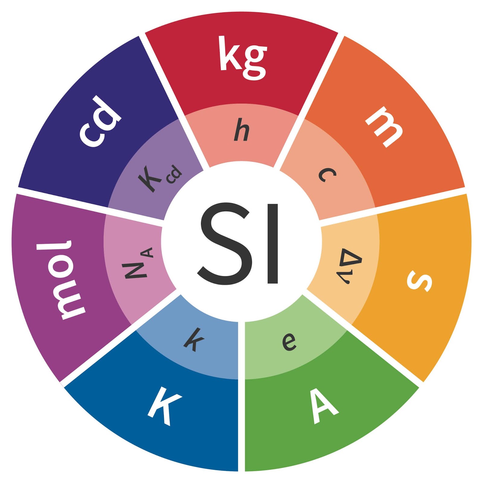
The SI logo, produced by the
International Bureau of Weights and Measures.

First let’s see where the seven base units appear in IPMB. Then we’ll examine the seven defining constants.

kilogram

The most basic units of the SI system are so familiar that Russ and I don’t bother defining them. The kilogram (mass, kg) appears throughout IPMB, but especially in Chapter 1, where density plays a major role in our analysis of fluid dynamics.

meter

We define the meter (distance, m) in Chapter 1 when discussing distances and scales: “The basic unit of length in the metric system is the meter (m): about the height of a 3-year-old child.” Both the meter and the kilogram are critical when discussing scaling in Chapter 2.

second

The second (time, s) is another unit that’s so basic Russ and I take it for granted. It plays a particularly large role in Chapter 10 when discussing nonlinear dynamics.

ampere

The SI system becomes more complicated when you add electrical units. IPMB defines the ampere (electrical current, A) in Section 6.8 about current and Ohm’s law: “The units of the current are C s⁻¹ [C is the unit of charge, a coulomb] or amperes (A) (sometimes called amps).”

kelvin

The unit for absolute temperature—the kelvin (temperature, K)—plays a central role in Chapter 3 of IPMB, when describing thermodynamics.

mole

The mole (number of molecules, mol) appears in Chapter 3 when relating microscopic quantities (Boltzmann’s constant, elementary charge) to macroscopic quantities (the gas constant, the Faraday). John Wikswo and I have introduced a name for a mole of differential equations (the leibniz), but the International Bureau of Weights and Measures inexplicably did not add it to their logo.

candela

Russ and I introduce the candela (luminous intensity, cd) in Section 14.12 of IPMB, when comparing radiometry to photometry: “The number of lumens per steradian is the luminous intensity, in lm sr⁻¹. The lumen per steradian is also called the candela.” The steradian (the unit of solid angle) used to play a more central role in the SI system, but appears to have been demoted.

Now we examine the seven constants that define these units.

Planck’s constant

In IPMB, the main role of Planck’s constant (h, 6.626 × 10⁻³⁴ J s) is to relate the frequency and energy of a photon. Quantum mechanics doesn’t play a major role in IPMB, so Planck’s constant appears less often than you might expect.

speed of light

Like quantum mechanics, relativity does not take center stage in IPMB, so the speed of light (c, 2.998 × 10⁸ m s⁻¹) appears rarely. We use it in Chapter 14 when relating the frequency of light to its wavelength, and in Chapter 17 when relating the mass of an elementary particle to its energy.

cesium hyperfine frequency

The cesium hyperfine frequency (Δν, 9.192 × 10⁹ Hz) defines the second. It never appears in IPMB. Why cesium? Why this particular atomic transition? I don’t know.

elementary charge

The elementary charge (e, 1.602 × 10⁻¹⁹ C) is used throughout IPMB, but is particularly important in Chapter 6 about bioelectricity.

Boltzmann’s constant

Boltzmann’s constant (k_B, 1.381 × 10⁻²³ J K⁻¹) appears primarily in Chapter 3 of IPMB, but also anytime Russ and I mention the Boltzmann factor.

Avogadro’s number

Like Boltzmann’s constant, Avogadro’s number (N_A, 6.022 × 10²³ mol⁻¹) shows up first in Chapter 3.

luminous efficacy

The luminous efficacy (K_cd, 683 lm W⁻¹) appears in Chapter 14 of IPMB: “The ratio P_v/P at 555 nm is the luminous efficacy for photopic vision, K_m = 683 lm W⁻¹.” I find this constant to be different from all the others. It’s a prime number specified to only three digits. Suppose a society of intelligent beings evolved on another planet. Their physicists would probably measure a set of constants similar to ours, and once we figured out how to convert units we would get the same values for six of the constants. The luminous efficacy, however, would depend on the physiology of their eyes (assuming they even have eyes). Perhaps I make too much about this. Perhaps the luminous efficacy merely defines the candela, just as Avogardo’s number defines the mole and Boltzmann’s constant defines the kelvin. Still, to me it has a different feel.

You can learn more about the SI units and constants in the International Bureau of Weights and Measures’ SI brochure. I’m fond of the SI logo, which reminds me of the circle of fifths. If you’re new to the metric systems, you might want to paste the logo into your copy of Intermediate Physics for Medicine and Biology; I suggest placing it in the white space on page 1, just above Table 1.1.

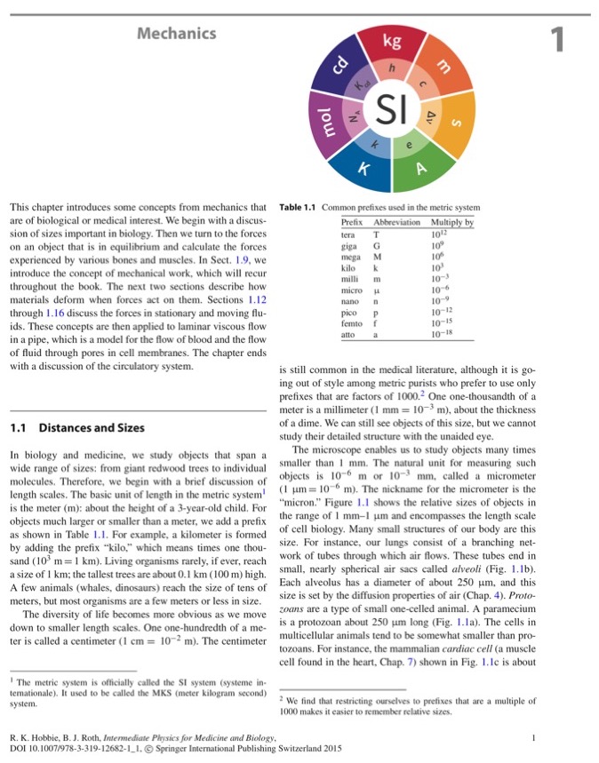
Page 1 of Intermediate Physics for Medicine and Biology,
with the SI Logo added at the top.

Free Convection and the Origin of Life

Free convection is an important process in fluid dynamics. Yet Russ Hobbie and I rarely discuss it in Intermediate Physics for Medicine and Biology. It appears only once, in a homework problem analyzing Rayleigh-Benard convection cells.

How does free convection work? If water is heated from below, it expands as it becomes hotter, reducing its density. Less dense water is buoyant and rises. As the water moves away from the source of heat, it cools, becomes denser, and sinks. The process then repeats. The fluid flow caused by all this rising, sinking, heating, and cooling is what’s known as free convection. One reason Russ and I don’t dwell on this topic is that our body is isothermal. You need a temperature gradient to drive convection.

“Thermal Habitat for RNA Amplification and Accumulation,”
by Salditt et al. (Phys. Rev. Lett., 125:048104, 2020).

Is free convection ever important in biology? According to a recent article in Physical Review Letters (Volume 125, Article Number 048104) by Annalena Salditt and her coworkers (“Thermal Habitat for RNA Amplification and Accumulation”), free convection may be responsible for the origin of life!

Many scientists believe early life was based on ribonucleic acid, or RNA, rather than DNA and proteins. RNA replication is aided by temperature oscillations, which allow the double-stranded RNA to separate and make complementary copies (hot), and then accumulate without being immediately degraded (cold). Molecules moving with water during free convection undergo such a periodic heating and cooling. One more process is needed, called thermophoresis, which causes long strands of RNA to move from hot to cold regions preferentially compared to short strands. Salditt et al. write

The interplay of convective and thermophoretic transport resulted in a length-dependent net transport of molecules away from the warm temperature spot. The efficiency of this transport increased for longer RNAs, stabilizing them against cleavage that would occur at higher temperatures.

Where does free convection happen? Around hydrothermal vents at the bottom of the ocean.

A natural setting for such a heat flow could be the dissipation of heat across volcanic or hydrothermal rocks. This leads to temperature differences over porous structures of various shapes and lengths.

The authors conclude

The search for the origin of life implies finding a location for informational molecules to replicate and undergo Darwinian evolution against entropic obstacles such as dilution and spontaneous degradation. The experiments described here demonstrate how a heat flow across a millimeter-sized, water-filled porous rock can lead to spatial separation of molecular species resulting in different reaction conditions for different species. The conditions inside such a compartment can be tuned according to the requirements of the partaking molecules due to the scalable nature of this setting. A similar setting could have driven both the accumulation and RNA-based replication in the emergence of life, relying only on thermal energy, a plausible geological energy source on the early Earth. Current forms of RNA polymerase ribozymes can only replicate very short RNA strands. However, the observed thermal selection bias toward long RNA strands in this system could guide molecular evolution toward longer strands and higher complexity.

You can learn more about this research from a focus article in Physics, an online magazine published by the American Physical Society.

Salditt et al.’s article provides yet another example of why I find the interface of physics and biology is so fascinating.

Tests for Human Perception of 60 Hz Moderate Strength Magnetic Fields

The first page of “Tests for Human Perception
of 60 Hz Moderate Strength Magnetic Fields,”
by Tucker and Schmitt (IEEE Trans. Biomed. Eng.
25:509-518, 1978).

In Chapter 9 of Intermediate Physics for Medicine and Biology, Russ Hobbie and I discuss possible effects of weak external electric and magnetic fields on the body. In a footnote, we write

Foster (1996) reviewed many of the laboratory studies and described cases where subtle cues meant the observers were not making truly “blind” observations. Though not directly relevant to the issue under discussion here, a classic study by Tucker and Schmitt (1978) at the University of Minnesota is worth noting. They were seeking to detect possible human perception of 60-Hz magnetic fields. There appeared to be an effect. For 5 years they kept providing better and better isolation of the subject from subtle auditory clues. With their final isolation chamber, none of the 200 subjects could reliably perceive whether the field was on or off. Had they been less thorough and persistent, they would have reported a positive effect that does not exist.

In this blog, I like to revisit articles that we cite in IPMB.

Robert Tucker and Otto Schmitt (1978) “Tests for Human Perception of 60 Hz Moderate Strength Magnetic Fields.” IEEE Transactions on Biomedical Engineering, Volume 25, Pages 509-518.

The abstract of their paper states

After preliminary experiments that pointed out the extreme cleverness with which perceptive individuals unintentionally used subtle auxiliary clues to develop impressive records of apparent magnetic field detection, we developed a heavy, tightly sealed subject chamber to provide extreme isolation against such false detection. A large number of individuals were tested in this isolation system with computer randomized sequences of 150 trials to determine whether they could detect when they were, and when they were not, in a moderate (7.5-15 gauss rms) alternating magnetic field, or could learn to detect such fields by biofeedback training. In a total of over 30,000 trials on more than 200 persons, no significantly perceptive individuals were found, and the group performance was compatible, at the 0.5 probability level, with the hypothesis that no real perception occurred.

The Tucker-Schmitt study illustrates how observing small effects can be a challenge. Their lesson is valuable, because many weak-field experiments are subject to systematic errors that provide an illusion of a positive result. Near the start of their article, Tucker and Schmitt write

We quickly learned that some individuals are incredibly skillful at sensing auxiliary non-magnetic clues, such as coil hum associated with field, so that some “super perceivers” were found who seemed to sense the fields with a statistical probability as much as 10^–30 against happening by chance. A vigorous campaign had then to be launched technically to prevent the subject from sensing “false” clues while leaving him completely free to exert any real magnetic perceptiveness he might have.

Few authors are as forthright as Tucker and Schmitt when recounting early, unsuccessful experiments. Yet, their tale shows how experimental scientists work.

Early experiments, in which an operator visible to the test subject controlled manually, according to a random number table, whether a field was to be applied or not, alerted us to the necessity for careful isolation of the test subject from unintentional clues from which he could consciously, or subconsciously, deduce the state of coil excitation. No poker face is good enough to hide, statistically, knowledge of a true answer, and even such feeble clues as changes in building light, hums, vibrations and relay clatter are converted into low but significant statistical biases.

IPMB doesn’t teach experimental methods, but all scientists must understand the difference between systematic and random errors. Uncertainty from random errors is suppressed by taking additional data, but eliminating systematic errors may require you to redesign your experiment.

In a first round of efforts to prevent utilization of such clues, the control was moved to a remote room and soon given over to a small computer. A “fake” air-core coil system, remotely located but matched in current drain and phase angle to the real large coil system was introduced as a load in the no-field cases. An acoustically padded cabinet was introduced to house the experimental subject, to isolate him from sound and vibration. Efforts were also made to silence the coils by clamping them every few centimeters with plastic ties and by supporting them on air pocket packing material. We tried using masking sound and vibrations, but soon realized that this might also mask real perception of magnetic fields.

Designing experiments is fun; you get to build stuff in a machine shop! I imagine Tucker and Schmitt didn’t expect they would have this much fun. Their initial efforts being insufficient, they constructed an elaborate cabinet to perform their experiments in.

This cabinet was fabricated with four layers of 2 in plywood, full contact epoxy glued and surface coated into a monolithic structure with interleaved corners and fillet corner reinforcement to make a very rigid heavy structure weighing, in total, about 300 kg. The structure was made without ferrous metal fastening and only a few slender brass screws were used. The door was of similar epoxyed 4-ply construction but faced with a thin bonded melamine plastic sheet. The door was hung on two multi-tongue bakelite hinges with thin brass pins. The door seals against a thin, closed-cell foam-rubber gasket, and is pressure sealed with over a metric ton of force by pumping a mild vacuum inside the chamber of means of a remote acoustically silenced hose-connected large vacuum-cleaner blower. The subject received fresh air through a small acoustic filter inlet leak that also assures sufficient air flow to cool the blower. The chosen “cabin altitude” at about 2500 ft above ambient presented no serious health hazard and was fail-safe protected.

An experimental scientist must be persistent. I remember learning that lesson as a graduate student when I tried for weeks to measure the magnetic field of a single nerve axon. I scrutinized every part of the experiment and fixed every problem I could find, but I still couldn’t measure an action current. Finally, I realized the coaxial cable connecting the nerve to the stimulator was defective. It was a rookie mistake, but I was tenacious and ultimately figured it out. Tucker and Schmitt personify tenacity.

As still more isolation seemed necessary to guarantee practically complete exclusion of auxiliary acoustic and mechanical clues, an extreme effort was made to improve, even further, the already good isolation. The cabinet was now hung by aircraft “Bungee” shock cord running through the ceiling to roof timbers. The cabinet was prevented from swinging as a pendulum by four small non-load-bearing lightly inflated automotive type inner tubes placed between the floor and the cabinet base. Coils already compliantly mounted to isolate intercoil force vibration were very firmly reclamped to discourage intracoil “buzzing.” The cabinet was draped inside with sound absorbing material and the chair for the subject shock-mounted with respect to the cabinet floor. The final experiments, in which minimal perception was found, were done with this system.

Once Tucker and Schmitt heroically eliminated even the most subtle cues about the presence of a magnetic field, subjects could no longer detect whether or not a magnetic field was present. People can’t perceive 60-Hz, 0.0015-T magnetic fields.

Russ and I relegate this tale to a footnote, but it’s an important lesson when analyzing the effects of weak electric and magnetic fields. Small systematic errors abound in these experiments, both when studying humans and when recording from cells in a dish. Experimentalists must ruthlessly design controls that can compensate for or eliminate confounding effects. The better the experimentalist, the more doggedly they root out systematic errors. One reason the literature on the biological effects of weak fields is so mixed may be that few experimentalists take the time to eradicate all sources of error.

Tucker and Schmitt’s experiment is a lesson for us all.

Physics World: Medical Physics

I subscribe to a weekly newsletter from Physics World about medical physics. This newsletter and its associated website (physicsworld.com/c/medical-physics) replace what used to be medicalphysicsweb.org. Like medicalphysicsweb, the newsletter is edited by Tami Freeman, which means the quality remains high. It’s one of the best ways to learn what’s new in medical physics.

On the website you find videos, podcasts, research updates, webinars, interviews, career advice, and job ads related to medical physics. You may find it almost as useful as hobbieroth.blogspot.com! Seriously, it has more and better content than this blog, but I suspect it has more resources behind it. In any event, both cost you the same: nothing. Sign up for an account at Physics World, then subscribe to the medical physics weekly newsletter. You won’t regret it.

Below is a sampler; some videos from Physics World that readers of Intermediate Physics for Medicine and Biology might find useful or interesting. Enjoy!

What are the benefits of proton therapy.

https://www.youtube.com/watch?v=PVWQ-VvL4ug

Reality check: Covid-19 and UV disinfection.

https://www.youtube.com/watch?v=eWNfqZf3h8o

How neutrons can help in the Covid-19 pandemic.

https://www.youtube.com/watch?v=DgvExXzQDg4&t=34s

The curious case of the porpoises and the wind farm.

https://www.youtube.com/watch?v=PhLqDBc4jcw

Faces of physics: human organs on a chip.

https://www.youtube.com/watch?v=p7vBPBHmmN4&amplist=PLdGQlH2iiDje18Qfm9SbfiitDyqtJhAwb

An S1 Gradient of Refractoriness is Not Essential for Reentry Induction by an S2 Stimulus

Sometimes the shortest papers are my favorites. Take, for example, an article that I published twenty years ago last month: a two-page communication in the IEEE Transactions on Biomedical Engineering titled “An S1 Gradient of Refractoriness is Not Essential for Reentry Induction by an S2 Stimulus” (Volume 47, Pages 820–821, 2000). It analyzes the electrical stimulation of cardiac tissue, and focuses on the mechanism for inducing an arrhythmia.

The introduction is two short paragraphs (a mere hundred words). The first puts the work in context.

Successive stimulation (S1, then S2) of cardiac tissue can induce reentry. In many cases, an S1 stimulus triggers a propagating action potential that creates a gradient of refractoriness. The S2 stimulus then interacts with this S1 refractory gradient, causing reentry. Many theoretical and experimental studies of reentry induction are variations on this theme [1]–[9].

When I wrote this communication, the critical point hypothesis was a popular explanation for how to induce reentry in cardiac tissue. I cited nine papers discussing this hypothesis, but I associate it primarily with the books of Art Winfree and the experiments of Ray Ideker.

The critical point hypothesis.

The figure above illustrates the critical point hypothesis. A first (S1) stimulus is applied to the right edge of the tissue, launching a planar wavefront that propagates to the left (arrow). By the time of the upper snapshot, the tissue on the right (purple) has returned to rest and recovered excitability, while the tissue on the left (red) remains refractory. The green line represents the boundary between refractory and excitable regions: the line of critical refractoriness.

The lower snapshot is immediately after a second (S2) stimulus is applied through a central cathode (black dot). The tissue near the cathode experiences a strong stimulus above threshold (yellow), while the remaining tissue experiences a weak stimulus below threshold. The green curve represents the boundary between the above-threshold and below-threshold regions: the circle of critical stimulus. S2 only excites tissue that is excitable and has a stimulus above threshold (inside the circle on the right). It launches a wave front that propagates to the right, but cannot propagate to the left because of refractoriness. Only when the refractory tissue recovers excitability will the wave front begin to propagate leftward (curved arrow). Critical points (blue dots) are located where the line of critical refractoriness intersects the circle of critical stimulus. Two spiral waves—a type of cardiac arrhythmia where a wave front circles around a critical point, chasing its tail—rotate clockwise on the bottom and counterclockwise on the top.

A beautiful paper from Ideker’s lab provides evidence supporting the critical point hypothesis: N. Shibata, P.-S. Chen, E. G. Dixon, P. D. Wolf, N. D. Danieley, W. M. Smith, and R. E. Ideker (1988) “Influence of Shock Strength and Timing on Induction of Ventricular Arrhythmias in Dogs,” American Journal of Physiology, Volume 255, Pages H891–H901.

The second paragraph of my communication begins with a question.

Is the S1 gradient of refractoriness essential for the induction of reentry? In this communication, my goal is to show by counterexample that the answer is no. In my numerical simulation, the transmembrane potential is uniform in space before the S2 stimulus. Nevertheless, the stimulus induces reentry.

The critical point hypothesis implies the answer is yes; without a refractory gradient there is no line of critical refractoriness, no critical point, no spiral wave, no reentry. Yet I claimed that the gradient of refractoriness is not essential. To explain why, we must consider what happens following the second stimulus.

Cathode break excitation.

The tissue is depolarized (D, yellow) under the cathode but is hyperpolarized (H, purple) in adjacent regions along the fiber direction on each side of the cathode, often called virtual anodes. Hyperpolarization lowers the membrane potential toward rest, shortening the refractory period (deexcitation) and carving out an excitable path. When S2 ends, the depolarization under the cathode diffuses into the newly excitable tissue (dashed arrows), launching a wave front that propagates initially in the fiber direction (solid arrows): break excitation. Only after the surrounding tissue recovers excitability does the wave front begin to rotate back, as if there were four critical points: quatrefoil reentry.

Russ Hobbie and I discuss break excitation in a homework problem in Chapter 7 of Intermediate Physics for Medicine and Biology.

Problem 48. During stimulation of cardiac tissue through a small anode, the tissue under the electrode and in the direction perpendicular to the myocardial fibers is hyperpolarized, and adjacent tissue on each side of the anode parallel to the fiber direction is depolarized. Imagine that just before this stimulus pulse is turned on the tissue is refractory. The hyperpolarization during the stimulus causes the tissue to become excitable. Following the end of the stimulus pulse, the depolarization along the fiber direction interacts electrotonically with the excitable tissue, initiating an action potential (break excitation). (This type of break excitation is very different than the break excitation analyzed on page 181.)

(a) Sketch pictures of the transmembrane potential distribution during the stimulus. Be sure to indicate the fiber direction, the location of the anode, the regions that are depolarized and hyperpolarized by the stimulus, and the direction of propagation of the resulting action potential.

(b) Repeat the analysis for break excitation caused by a cathode instead of an anode. For a hint, see Wikswo and Roth (2009).

Now we come to the main point of the communication; the reason I wrote it. Look at the first snapshot in the illustration above, the one labeled S1 that occurs just before the S2 stimulus. The tissue is all red. It is uniformly refractory. The S1 action potential has no gradient of refractoriness, yet reentry occurs. This is the counterexample that proves the point: a gradient of refractoriness is not essential.

The communication contains one figure, showing the results of a calculation based on the bidomain model. The time in milliseconds after S1 is in the upper right corner of each panel. S1 was applied uniformly to the entire tissue, so at 70 ms the refractoriness is uniform. The 80 ms frame is during S2. Subsequent frames show break excitation the development of reentry.

An illustration based on Fig. 1 in “An S1 Gradient of Refractoriness is Not Essential for Reentry Induction by an S2 Stimulus” (IEEE TBME, 47:820–821, 2000). It is the same as the figure in the communication, except the color and quality are improved.

The communication concludes:

My results support the growing realization that virtual electrodes, hyperpolarization, deexcitation, and break stimulation may be important during reentry induction [8], [9], [14], [15], [21]–[24]. An S1 gradient of refractoriness may underlie reentry induction in many cases [1]–[6], but this communication provides a counterexample demonstrating that an S1 gradient of refractoriness is not necessary in every case.

This is a nice calculation, but is it consistent with experiment? Look at Y. Cheng, V. Nikolski, and I. R. Efimov (2000) “Reversal of Repolarization Gradient Does Not Reverse the Chirality of Shock-Induced Reentry in the Rabbit Heart,” Journal of Cardiovascular Electrophysiology, Volume 11, Pages 998–1007. These researchers couldn’t produce uniform refractoriness, so they did the next best thing: repeated the experiment using S1 wave fronts propagating in different directions. They always obtained the same result, independent of the location and timing of the critical line of refractoriness.

Does this calculation mean the critical point hypothesis is wrong? No. See my paper with Natalia Trayanova and her student Annette Lindblom (“The Role of Virtual Electrodes in Arrhythmogenesis: Pinwheel Experiment Revisited,” Journal of Cardiovascular Electrophysiology, Volume 11, Pages 274-285, 2000) to examine how this view of reentry can be reconciled with the critical point hypothesis.

One of the best things about this calculation is that you don’t need a fancy computer to demonstrate that the S1 gradient of refracoriness is not essential; A simple cellular automata will do. The figure below sums it up (look here if you don’t understand).

A cellular automata demonstrating that an S1 gradient of refractoriness is not essential for reentry induction by an S2 stimulus.

Dreyer’s English

Dreyer’s English,
by Benjamin Dreyer.

In this blog I’ve reviewed several books about writing (On Writing Well, Plain Words, Do I Make Myself Clear?). I do this because many readers of Intermediate Physics for Medicine and Biology will become writers of scientific articles, grant proposals, or textbooks. Today, I review the funniest of these books: Dreyer’s English: An Utterly Correct Guide to Clarity and Style. If you believe a book about writing must be dull, read Dreyer’s English; you’ll change your mind.

At the start of his book, Benjamin Dreyer writes

Here’s your first challenge: Go a week without writing

• Very

• Rather

• Really

• Quite

• In fact

And you can toss in—or, that is, toss out—“just” (not in the sense of “righteous” but in the sense of “merely”) and “so” (in the “extremely” sense, through as conjunctions go it’s pretty disposable too).

Oh yes: “pretty.” As in “pretty tedious.” Or “pretty pedantic.” Go ahead and kill that particular darling.

And “of course.” That’s right out. And “surely.” And “that said.”

And “actually”? Feel free to go the rest of your life without another “actually.”

If you can last a week without writing any of what I’ve come to think of as the Wan Intensifiers and Throat Clearers—I wouldn’t ask you to go a week without saying them; that would render most people, especially British people, mute—you will at the end of that week be a considerably better writer than your were at the beginning.

Let’s go through Intermediate Physics for Medicine and Biology and see how often Russ Hobbie and I use these empty words.

Very

I tried to count how many times Russ and I use “very” in IPMB. I thought using the pdf file and search bar would make this simple. However, when I reached page 63 (a tenth of the way through the book) with 30 “very”s I quit counting, exhausted. Apparently “very” appears about 300 times.

Sometimes our use of “very” is unnecessary. For instance, “Biophysics is a very broad subject” would sound better as “Biophysics is a broad subject,” and “the use of a cane can be very effective” would be more succinct as “the use of a cane can be effective.” In some cases, we want to stress that something is extremely small, such as “the nuclei of atoms (Chap. 17) are very small, and their sizes are measured in femtometers (1 fm = 10⁻¹⁵ m).” If I were writing the book again, I would consider replacing “very small” by “tiny.” In other cases, a “very” seems justified to me, as in “the resting concentration of calcium ions, [Ca⁺⁺], is about 1 mmol l⁻¹ in the extracellular space but is very low (10⁻⁴ mmol l⁻¹) inside muscle cells,” because inside the cell the calcium concentration is surprisingly low (maybe we should have replaced “very” by “surprisingly”). Finally, sometimes we use “very” in the sense of finding the limit of a function as a variable goes to zero or infinity, as in “for very long pulses there is a minimum current required to stimulate that is called rheobase.” To my ear, this is a legitimate “very” (if infinity isn’t very big, then nothing is). Nevertheless, I concede that we could delete most “very”s and the book would be improved.

Rather

I counted 33 “rather”s in IPMB. Usually Russ and I use “rather” in the sense of “instead” (“this rather than that”), as in “the discussion associated with Fig. 1.5 suggests that torque is taken about an axis, rather than a point.” I’m assuming Dreyer won’t object to this usage (but you know what happens when you assume...). Only occasionally do we use “rather” in its rather annoying sense: “the definition of a microstate of a system has so far been rather vague,” and “this gives a rather crude image, but we will see how to refine it.”

Really

Russ and I do really well, with only seven “really”s. Dreyer or no Dreyer, I’m not getting rid of the first one: “Finally, thanks to our long-suffering families. We never understood what these common words really mean, nor the depth of our indebtedness, until we wrote the book.”

Quite

I quit counting “quite” part way through IPMB. The first half contains 33, so we probably have sixty to seventy in the whole book. Usually we use “quite” in the sense of “very”: “in the next few sections we will develop some quite remarkable results from statistical mechanics,” or “there is, of course, something quite unreal about a sheet of charge extending to infinity.” These could be deleted with little loss. I would keep this one: “while no perfectly selective channel is known, most channels are quite selective,” because, in fact, I’m really quite amazed how so very selective these channels are. I would also keep “the lifetime in the trapped state can be quite long—up to hundreds of years,” because hundreds of years for a trapped state! Finally, I’m certain our students would object if we deleted the “quite” in “This chapter is quite mathematical.”

In Fact

I found only 24 “in fact”s, which isn’t too bad. One’s in a quote, so it’s not our fault. All the rest could go. The worst one is “This fact is not obvious, and in fact is true only if…”. Way too much “fact.”

Just

Russ and I use “just” a lot. I found 39 “just”s in the first half of the book, so we probably have close to eighty in all. Often we use “just” in a way that is neither “righteous” nor “merely,” but closer to “barely.” For instance, “the field just outside the cell is roughly the same as the field far away.” I don’t know what Dreyer would say, but this usage is just alright with me.

So

Searching the pdf for “so” was difficult; I found every “also,” “some,” “absorb,” “solute,” “solution,” “sodium,” “source,” and a dozen other words. I’m okay (and so is Dreyer) with “so” being used as a conjunction to mean “therefore,” as in “only a small number of pores are required to keep up with the rate of diffusion toward or away from the cell, so there is plenty of room on the cell surface for many different kinds of pores and receptor sites.” I also don’t mind the “so much…that” construction, such as “the distance 0.1 nm (100 pm) is used so much at atomic length scales that it has earned a nickname: the angstrom.” I doubt Russ and I ever use “so” in the sense of “dude, you are so cool,” but I got tired of searching so I’m not sure.

Pretty

Only one “pretty”: “It is interesting to compare the spectral efficiency function with the transmission of light through 2 cm of water (Fig. 14.36). The eye’s response is pretty well centered in this absorption window.” We did a pretty good job with this one.

Of Course

I didn’t expect to find many “of course”s in our book, but there are fourteen of them. For example, “both assumptions are wrong, of course, and later we will improve upon them.” I hope, of course, that readers are not offended by this. We could do without most or all of them.

Surely

None. Fussy Mr. Dreyer surely can’t complain.

That Said

None.

Actually

I thought Russ and I would do okay with “actually,” but no; we have 38 of them. Dreyer says that “actually…serves no purpose I can think of except to irritate.” I’m not so sure. We sometimes use it in the sense of “you expect this, but actually get that.” For example, “the total number of different ways to arrange the particles is N! But if the particles are identical, these states cannot be distinguished, and there is actually only one microstate,” and “we will assume that there is no buildup of concentration in the dialysis fluid… (Actually, proteins cause some osmotic pressure difference, which we will ignore.)” Dreyer may not see its purpose, but I actually think this usage is justified. I admit, however, that it’s a close call, and most “actually”s could go.

Books I keep on my desk
(except for Dreyer’s English, which is a
library copy; I need to buy my own).

I was disappointed to find so many appearances of “very,” “rather,” “really,” “quite,” “in fact,” “just,” “so,” “pretty,” “of course,” “surely,” “that said,” and “actually” in Intermediate Physics for Medicine and Biology. We must do better.

Dreyer concludes

For your own part, if you can abstain from these twelve terms for a week, and if you read not a single additional word of this book—if you don’t so much as peek at the next page—I’ll be content.

 The next page says

Well, no.

But it sounded good.

Benjamin Dreyer and Rachel Joyce on grammar and language.
https://www.youtube.com/watch?v=t4W26oC28Ik

Eric Betzig, Biological Physicist

Important advances in fluorescence microscopy highlight the interaction of physics and biology. This effort is led by Eric Betzig of Berkeley, winner of the 2014 Chemistry Nobel Prize. Betzig obtained his bachelor’s and doctorate degrees in physics, and only later began collaborating with biologists. He is a case-study for how physicists can contribute to the life sciences, a central theme of Intermediate Physics for Medicine and Biology.

If you want to learn about Betzig’s career and work, watch the video at the bottom of this post. In it, he explains how designing a new microscope requires trade-offs between spatial resolution, temporal resolution, imaging depth, and phototoxicity. Many super-resolution fluorescence microscopes (having extraordinarily high spatial resolution, well beyond the diffraction limit) require intense light sources, which cause bleaching or even destruction of the fluorophore. This phototoxicity arises because the excitation light illuminates the entire sample, although much of it doesn’t contribute to the image (as in a confocal microscope). Moreover, microscopes with high spatial resolution must acquire a huge amount of data to form an image, which makes them too slow to follow the rapid dynamics of a living cell.

Eric Betzig’s explanation of the trade-offs between spatial resolution, temporal resolution, imaging depth, and phototoxicity.

Betzig’s key idea is to trade lower spatial resolution for improved temporal resolution and less phototoxicity, creating an unprecedented tool for imaging structure and function in living cells. The figure below illustrates his light-sheet fluorescence microscope.

A light-sheet fluorescence microscope.

The sample (red) is illuminated by a thin sheet of short-wavelength excitation light (blue). This light excites fluorescent molecules in a thin layer of the sample; the position of the sheet can be varied in the z direction, like in MRI. For each slice, the long-wavelength fluorescent light (green) is imaged in the x and y directions by the microscope with its objective lens.

The advantage of this method is that only those parts of the sample to be imaged are exposed to excitation light, reducing the total exposure and therefore the phototoxicity. The thickness of the light sheet can be adjusted to set the depth resolution. The imaging by the microscope can be done quickly, increasing its temporal resolution.

A disadvantage of this microscope is that the fluorescent light is scattered as it passes through the tissue between the light sheet and the objective. However, the degradation of the image can be reduced with adaptive optics, a technique used by astronomers to compensate for scattering caused by turbulence in the atmosphere.

Listen to Betzig describe his career and research in the hour-and-a-half video below. If you don’t have that much time, or you are more interested in the microscope than in Betzig himself, watch the eight-minute video about recent developments in the Advanced Bioimaging Center at Berkeley. It was produced by Seeker, a media company that makes award-winning videos to explain scientific innovations.

Enjoy!

A 2015 talk by Eric Betzig about imaging life at high spatiotemporal resolution.

https://www.youtube.com/watch?v=2R2ll9SRCeo

“Your Textbooks Are Wrong, This Is What Cells Actually Look Like.” Produced by Seeker.

https://www.youtube.com/watch?v=9euW5iCjKDo

The Berkeley Physics Course

In Intermediate Physics for Medicine and Biology, Russ Hobbie and I cite two volumes of the Berkeley Physics Course: Volume II about electricity and magnetism, and Volume V about statistical mechanics. This five-volume set provides a wonderful introduction to physics. Its preface states

This is a two-year elementary college physics course for students majoring in science and engineering. The intention of the writers has been to present elementary physics as far as possible in the way in which it is used by physicists working on the forefront of their field. We have sought to make a course which would vigorously emphasize the foundations of physics. Our specific objectives were to introduce coherently into an elementary curriculum the ideas of special relativity, of quantum physics, and of statistical physics.

The course is intended for any student who has had a physics course in high school. A mathematics course including the calculus should be taken at the same time as this course….

The five volumes of the course as planned will include:

I. Mechanics (Kittel, Knight, Ruderman)

II. Electricity and Magnetism (Purcell)

III. Waves and Oscillations (Crawford)

IV. Quantum Physics (Wichmann)

V. Statistical Physics (Reif)

 ...The initial course activity led Alan M. Portis to devise a new elementary physics laboratory.

Statistical Physics,
Volume 5 of the Berkeley Physics Course,
by Frederick Reif.

Chapter 3 of IPMB is modeled in part on Volume V by Frederick Reif.

Preface to Volume V

The last volume of the Berkeley Physics Course is devoted to the study of large-scale (i.e., macroscopic) systems consisting of many atoms or molecules: thus it provides an introduction to the subjects of statistical mechanics, kinetic theory, thermodynamics, and heat…My aim has been … to adopt a modern point of view and to show, in as systematic and simple a way as possible, how the basic notions of atomic theory lead to a coherent conceptual framework capable of describing and predicting the properties of macroscopic systems.

I love Reif’s book, in part because of nostalgia: it’s the textbook I used in my undergraduate thermodynamics class at the University of Kansas. His Chapter 4 is similar to IPMB’s Chapter 3, where the concepts of heat transfer, absolute temperature, and entropy are shown to result from how the number of states depends on energy. Boltzmann’s factor is derived, and the two-state magnetic system important in magnetic resonance imaging is analyzed. Reif even has short biographies of famous scientists who worked on thermodynamics—such as Boltzmann, Kelvin, and Joule—which I think of as little blog posts built into the textbook. If you want more detail, Reif also has a larger book about statistical and thermal physics that we also cite in IPMB.

Electricity and Magnetism,
Volume 2 of the Berkeley Physics Course,
by Edward Purcell.

Russ and I sort of cite Edward Purcell’s Volume II of the Berkeley Physics Course. Earlier editions of IPMB cited it, but in the 5th edition we cite the book Electricity and Magnetism by Purcell and Morin (2013). It is nearly equivalent to Volume II, but is an update by an additional author. If you want to gain insight into electricity and magnetism, you should read Purcell.

Preface to Volume II

The subject of this volume of the Berkeley Physics Course is electricity and magnetism. The sequence of topics, in rough outline, is not unusual: electrostatics; steady currents; magnetic field; electromagnetic induction; electric and magnetic polarization in matter. However, our approach is different from the traditional one. The difference is most conspicuous in Chaps. 5 and 6 where, building on the work of Vol. I, we treat the electric and magnetic fields of moving charges as manifestations of relativity and the invariance of electric charge.

I love Purcell’s book, but introducing magnetism as a manifestation of special relativity is not the best way to teach the subject to students of biology and medicine. In IPMB we never adopt this view except in a couple teaser homework problems (8.5 and 8.26).

IPMB doesn’t cite Volumes I, III, or IV of the Berkeley Physics Course. If we did, where in the book would those citations be? Kittel, Knight, and Ruderman’s Volume I covers classical mechanics. They analyze the dynamics of particles in a cyclotron so that we could cite it in Chapter 8 of IPMB, and they describe the harmonic oscillator so we could cite it in our Chapter 10. Crawford’s Volume III on waves could be cited in Chapter 13 of IPMB about sound and ultrasound. Wichmann’s Volume IV on quantum mechanics would fit well in the first part of our Chapter 14 on atoms and light.

Do universities adopt the Berkeley Physics Course textbooks anymore? I doubt it. The series is out-of-date, having been published in the 1960s. The use of cgs rather than SI units makes the books seem old fashioned. The preface says it’s a two-year introduction to physics (five semesters, one semester for each book), while most schools offer a one-year (two-semester) sequence. The books don’t have the flashy color photos so common in modern introductory texts. Nevertheless, if you were introduced to physics through the Berkeley Physics Course, you would have a strong grasp of physics fundamentals, and would have more than enough preparation for a course based on Intermediate Physics for Medicine and Biology.

Atomic Accidents

Reading Atomic Accidents,
by Jim Mahaffey,
in my home office.

The Oakland University library has online access to the book Atomic Accidents: A History of Nuclear Meltdowns and Disasters, From the Ozark Mountains to Fukushima, by Jim Mahaffey. I’m glad they do; with the library still locked up because of the coronavirus pandemic, I wouldn’t have been able to check out a paper copy. The book is more about nuclear engineering than nuclear medicine, but the two fields intersect during nuclear accidents, so it’s relevant to readers of Intermediate Physics for Medicine and Biology.

In his introduction, Mahaffey compares the 20th century invention of nuclear power to the 19th century development of steam-powered trains. Then he writes

In this book we will delve into the history of engineering failures, the problems of pushing into the unknown, and bad luck in nuclear research, weapons, and the power industry. When you see it all in one place, neatly arranged, patterns seem to appear. The hidden, underlying problems may come into focus. Have we been concentrating all effort in the wrong place? Can nuclear power be saved from itself, or will there always be another problem to be solved? Will nuclear fission and its long-term waste destroy civilization, or will it make civilization possible?

Some of these disasters you have heard about over and over. Some you have never heard of. In all of them, there are lessons to be learned, and sometimes the lessons require multiple examples before the reality sinks in. In my quest to examine these incidents, I was dismayed to find that what I thought I knew, what I had learned in the classroom, read in textbooks, and heard from survivors could be inaccurate. A certain mythology had taken over in both the public and the professional perceptions of what really happened. To set the record straight, or at least straighter than it was, I had to find and study buried and forgotten original reports and first-hand accounts. With declassification at the federal level, ever-increasing digitization of old documents, and improvements in archiving and searching, it is now easier to see what really happened.

So here, Gentle Reader, is your book of train wrecks, disguised as something in keeping with our 21st century anxieties. In this age, in which we strive for better sources of electrical and motive energy, there exists a deep fear of nuclear power, which makes accounts of its worst moments of destruction that much more important. The purpose of this book is not to convince you that nuclear power is unsafe beyond reason, or that it will lead to the destruction of civilization. On the contrary, I hope to demonstrate that nuclear power is even safer than transportation by steam and may be one of the key things that will allow life on Earth to keep progressing; but please form your own conclusions. The purpose is to make you aware of the myriad ways that mankind can screw up a fine idea while trying to implement it. Don’t be alarmed. This is the raw, sometimes disturbing side of engineering, about which much of humanity has been kept unaware. You cannot be harmed by just reading about it.

That story of the latest nuclear catastrophe, the destruction of the Fukushima Daiichi plant in Japan, will be held until near the end. We are going to start slowly, with the first known incident of radiation poisoning. It happened before the discovery of radiation, before the term was coined, back when we were blissfully ignorant of the invisible forces of the atomic nucleus.

I’ll share just one accident that highlights some of the issues with reactor safety discussed by Mahaffey. It took place at the Chalk River reactor in Ontario, Canada, about 300 miles northeast of Oakland University, as the crow flies.

I found several parallels between the Chalk River and Chernobyl accidents (readers might want to review my earlier post about Chernobyl before reading on). Both hinged on the design of the reactor, and in particular on the type of moderator used to slow neutrons. Both highlight how human error can overcome the most careful of safety designs. Their main difference is that Chalk River was a minor incident while Chernobyl was a catastrophe.

The Chalk River reactor began as a Canadian-British effort during World War II that operated in parallel to America’s Manhattan Project. It’s development has more in common with the plutonium-producing Hanford Site in Washington state than with the bomb-building laboratory in Los Alamos. After Enrico Fermi and his team built the first nuclear reactor in Chicago using graphite as the moderator, the Canadian-British team decided to explore moderation by heavy water. In 1944 they began to build a low-power experimental reactor along the Chalk River. For safety, the reactor has a scram consisting of heavy cadmium plates that would absorb neutrons and would lower into the reactor if a detector recorded too high of a neutron flux, shutting down nuclear fission. The energy production was controlled by raising and lowering the level of heavy water, which could be pumped into the reactor by pushing a switch. As a safety precaution, the pump would turn off after 10 seconds unless the switch was pushed again. To power up the reactor, the operator had to push the switch over and over.

In the summer of 1950 an accident occurred. Two physicists were going to test a new fuel rod design, so the reactor was shut down. The operator knew he would have to push the heavy water button many times to restart the reactor, so he began early, before the physicists were done installing the rod. Growing tired of repeatedly pushing the button, he shoved a wood chip into the switch so it was stuck on. Then the phone rang, and he was distracted by the call. The reactor went supercritical and the two physicists were doused with gamma radiation until the cadmium plates descended. Fortunately, the plates shut down the reactor before too much damage was done, and the physicists survived. Yet, the accident provides many lessons, including how human error can cause the best laid plans to go awry.

Later, a much larger reactor was built at Chalk River, and Mahaffey tells more horror stories about subsequent accidents, including one that required months of cleanup that was led in part by future President Jimmy Carter.

This story is a sample of what you’ll find in Atomic Accidents. Mahaffey describes all sorts of mishaps, from a sodium-cooled plutonium breeder reactor that in the 1960s that almost lost Detroit (Yikes, that's just down the road from where I sit writing this post), to a variety of incidents in which an atomic bomb (usually not armed) was damaged or lost, to the frightening Kyshtym disaster in 1957 at the Mayak plutonium production site in Russia. He ends the book by describing the better-known accidents at Three-Mile Island, Chernobyl, and Fukushima.

I didn’t realize how all-or-nothing an atomic reactor is. The nuclear fuel is below a critical mass and inert until it reaches a threshold of criticality, at which point it promptly releases a burst of energy and neutrons. Usually it doesn’t blow up like a bomb, because it typically melts before the chain reaction can reach truly explosive proportions. Mahaffey has all sorts of terrifying tales. One begins with a fissile material such as uranium-235 or plutonium-239 dissolved in water; A technician pores the water from one container to another with a more spherical shape, resulting in a flash of neutrons and gamma rays that deliver a lethal dose of radiation.

After scaring us all to death, Mahaffey ends on an upbeat note.

The dangers of continuing to expand nuclear power will always be there, and there could be another unexpected reactor meltdown tomorrow, but the spectacular events that make a compelling narrative may be behind us now. We have learned from each incident. As long as nuclear engineering can strive for new innovations and learn from its history of accidents and mistakes, the benefits that nuclear power can yield for our economy, society, and yes, environment will come.

Atomic Accidents reminded me of Henry Petroski’s wonderful To Engineer is Human: The Role of Failure in Successful Design. The thesis of both books is that you can learn more by examining how things fail than how things succeed. If you want to understand nuclear engineering, the best way is to study atomic accidents.

Pneumoencephalography

How did neuroradiologists image the brain before the invention of computed tomography and magnetic resonance imaging? They used a form of torture called pneumoencephalography. Perhaps the greatest contribution of CT and MRI—both discussed in Intermediate Physics for Medicine and Biology—was to make pneumoencephalography obsolete.

In their article “Evolution of Diagnostic Neuroradiology from 1904 to 1999,” (Radiology, Volume 217, Pages 309-318, 2000), Norman Leeds and Stephen Kieffer describe this odious procedure.

Pneumoencephalography was performed by successively injecting small volumes of air via lumbar puncture and then removing small volumes of cerebrospinalfluid with the patient sitting upright and the head flexed... Pneumoencephalography was used primarily to determine the presence and extent of posterior fossa or cerebellopontine angle tumors, pituitary tumors, and intraventricular masses... It was also used to rule out the presence of lesions affecting the cerebrospinal fluid spaces in patients with possible communicating hydrocephalus or dementia... After the injection of a sufficient quantity of air, the patient was rotated, somersaulted, or placed in a decubitus position to depict the entire ventricularsystem and subarachnoid spaces. These patients were often uncomfortable, developed severe headaches, and became nauseated or vomited.

In Chapter 7 of the book Radiology 101: The Basics and Fundamentals, Wilbur Smith shares this lurid tale.

The early brain imaging techniques… involved such gruesome activities as injecting air into the spinal canal (pneumoencephalography) and rolling the patient about in a specially devised torture chair. Few patients willingly returned for another one of those examinations!

In her book The Immortal Life of Henrietta Lacks, Rebecca Skloot writes

I later learned that while Elsie was at Crownsville, scientists often conducted research on patients there without consent, including one study titled “Pneumoencephalographic and skull X-ray studies in 100 epileptics.” Pneumoencephalography was a technique developed in 1919 for taking images of the brain, which floats in a sea of liquid. That fluid protects the brain from damage, but makes it very difficult to X-ray, since images taken through fluid are cloudy. Pneumoencephalography involved drilling holes into the skulls of research subjects, draining the fluid surrounding their brains, and pumping air or helium into the skull in place of the fluid to allow crisp X-rays of the brain through the skull. the side effects—crippling headaches, dizziness, seizures, vomiting—lasted until the body naturally refilled the skull with spinal fluid, which usually took two to three months. Because pneumoencephalography could cause permanent brain damage and paralysis, it was abandoned in the 1970s.

Russ Hobbie claims that the development of CT deserved the Nobel Peace Prize in addition to the Nobel Prize in Physiology or Medicine!

The application of physics to medicine and biology isn’t just to diagnose diseases that couldn’t be diagnosed before. It also can help replace barbaric procedures by ones that are more humane.

A scene from The Exorcist, in which Regan undergoes pneumoencephalography. 

https://www.youtube.com/watch?v=HBNdGOQ9Exk