On the website you find videos, podcasts, research updates, webinars, interviews, career advice, and job ads related to medical physics. You may find it almost as useful as hobbieroth.blogspot.com! Seriously, it has more and better content than this blog, but I suspect it has more resources behind it. In any event, both cost you the same: nothing. Sign up for an account at Physics World, then subscribe to the medical physics weekly newsletter. You won’t regret it.
The introduction is two short paragraphs (a mere hundred words). The first puts the work in context.
Successive stimulation (S1, then S2) of cardiac tissue can induce
reentry. In many cases, an S1 stimulus triggers a propagating action potential that creates a gradient of refractoriness. The S2 stimulus then
interacts with this S1 refractory gradient, causing reentry. Many theoretical
and experimental studies of reentry induction are variations on
this theme [1]–[9].
When I wrote this communication, the critical point hypothesis was a popular explanation for how to induce reentry in cardiac tissue. I cited nine papers discussing this hypothesis, but I associate it primarily with the books of Art Winfree and the experiments of Ray Ideker.
The critical point hypothesis.
The figure above illustrates the critical point hypothesis. A first (S1) stimulus is applied to the right edge of the tissue, launching a planar wavefront that propagates to the left (arrow). By the time of the upper snapshot, the tissue on the right (purple) has returned to rest and recovered excitability, while the tissue on the left (red) remains refractory. The green line represents the boundary between refractory and excitable regions: the line of critical refractoriness.
The lower snapshot is immediately after a second (S2) stimulus is applied through a central cathode (black dot). The tissue near the cathode experiences a strong stimulus above threshold (yellow), while the remaining tissue experiences a weak stimulus below threshold. The green curve represents the boundary between the above-threshold and below-threshold regions: the circle of critical stimulus. S2 only excites tissue that is excitable and has a stimulus above threshold (inside the circle on the right). It launches a wave front that propagates to the right, but cannot propagate to the left because of refractoriness. Only when the refractory tissue recovers excitability will the wave front begin to propagate leftward (curved arrow). Critical points (blue dots) are located where the line of critical refractoriness intersects the circle of critical stimulus. Two spiral waves—a type of cardiac arrhythmia where a wave front circles around a critical point, chasing its tail—rotate clockwise on the bottom and counterclockwise on the top.
The second paragraph of my communication begins with a question.
Is the S1 gradient of refractoriness essential for the induction of
reentry? In this communication, my goal is to show by counterexample
that the answer is no. In my numerical simulation, the transmembrane
potential is uniform in space before the S2 stimulus. Nevertheless, the
stimulus induces reentry.
The critical point hypothesis implies the answer is yes; without a refractory gradient there is no line of critical refractoriness, no critical point, no spiral wave, no reentry. Yet I claimed that the gradient of refractoriness is not essential. To explain why, we must consider what happens following the second stimulus.
Cathode break excitation.
The tissue is depolarized (D, yellow) under the cathode but is hyperpolarized (H, purple) in adjacent regions along the fiber direction on each side of the cathode, often called virtual anodes. Hyperpolarization lowers the membrane potential toward rest, shortening the refractory period (deexcitation) and carving out an excitable path. When S2 ends, the depolarization under the cathode diffuses into the newly excitable tissue (dashed arrows), launching a wave front that propagates initially in the fiber direction (solid arrows): break excitation. Only after the surrounding tissue recovers excitability does the wave front begin to rotate back, as if there were four critical points: quatrefoil reentry.
Problem 48. During stimulation of cardiac tissue through a
small anode, the tissue under the electrode and in the direction
perpendicular to the myocardial fibers is hyperpolarized,
and adjacent tissue on each side of the anode parallel to the
fiber direction is depolarized. Imagine that just before this
stimulus pulse is turned on the tissue is refractory. The hyperpolarization
during the stimulus causes the tissue to become
excitable. Following the end of the stimulus pulse, the depolarization
along the fiber direction interacts electrotonically
with the excitable tissue, initiating an action potential (break
excitation). (This type of break excitation is very different
than the break excitation analyzed on page 181.)
(a) Sketch pictures of the transmembrane potential distribution
during the stimulus. Be sure to indicate the fiber
direction, the location of the anode, the regions that are
depolarized and hyperpolarized by the stimulus, and the
direction of propagation of the resulting action potential.
(b) Repeat the analysis for break excitation caused by a
cathode instead of an anode. For a hint, see Wikswo and Roth (2009).
Now we come to the main point of the communication; the reason I wrote it. Look at the first snapshot in the illustration above, the one labeled S1 that occurs just before the S2 stimulus. The tissue is all red. It is uniformly refractory. The S1 action potential has no gradient of refractoriness, yet reentry occurs. This is the counterexample that proves the point: a gradient of refractoriness is not essential.
The communication contains one figure, showing the results of a calculation based on the bidomain model. The time in milliseconds after S1 is in the upper right corner of each panel. S1 was applied uniformly to the entire tissue, so at 70 ms the refractoriness is uniform. The 80 ms frame is during S2. Subsequent frames show break excitation the development of reentry.
An illustration based on Fig. 1 in “An S1 Gradient of Refractoriness is Not Essential for Reentry Induction by an S2 Stimulus” (IEEE TBME, 47:820–821, 2000). It is the same as the figure in the communication, except the color and quality are improved.
The communication concludes:
My results support the growing realization that virtual electrodes, hyperpolarization,
deexcitation, and break stimulation may be important
during reentry induction [8], [9], [14], [15], [21]–[24]. An S1 gradient
of refractoriness may underlie reentry induction in many cases [1]–[6],
but this communication provides a counterexample demonstrating that
an S1 gradient of refractoriness is not necessary in every case.
Does this calculation mean the critical point hypothesis is wrong? No. See my paper with Natalia Trayanova and her student Annette Lindblom (“The Role of Virtual Electrodes in Arrhythmogenesis: Pinwheel Experiment Revisited,” Journal of Cardiovascular Electrophysiology, Volume 11, Pages 274-285, 2000) to examine how this view of reentry can be reconciled with the critical point hypothesis.
One of the best things about this calculation is that you don’t need a fancy computer to demonstrate that the S1 gradient of refracoriness is not essential; A simple cellular automata will do. The figure below sums it up (look here if you don’t understand).
A cellular automata demonstrating that an S1 gradient of refractoriness is not essential for reentry induction by an S2 stimulus.
Here’s your first challenge: Go a week without writing
• Very
• Rather
• Really
• Quite
• In fact
And you can toss in—or, that is, toss out—“just” (not in the sense of “righteous” but in the sense of “merely”) and “so” (in the “extremely” sense, through as conjunctions go it’s pretty disposable too).
Oh yes: “pretty.” As in “pretty tedious.” Or “pretty pedantic.” Go ahead and kill that particular darling.
And “of course.” That’s right out. And “surely.” And “that said.”
And “actually”? Feel free to go the rest of your life without another “actually.”
If you can last a week without writing any of what I’ve come to think of as the Wan Intensifiers and Throat Clearers—I wouldn’t ask you to go a week without saying them; that would render most people, especially British people, mute—you will at the end of that week be a considerably better writer than your were at the beginning.
I tried to count how many times Russ and I use “very” in IPMB. I thought using the pdf file and search bar would make this simple. However, when I reached page 63 (a tenth of the way through the book) with 30 “very”s I quit counting, exhausted. Apparently “very” appears about 300 times.
Sometimes our use of “very” is unnecessary. For instance, “Biophysics is a very broad subject” would sound better as “Biophysics is a broad subject,” and “the use of a cane can be very effective” would be more succinct as “the use of a cane can be effective.” In some cases, we want to stress that something is extremely small, such as “the nuclei of atoms (Chap. 17) are very small, and their sizes are measured in femtometers (1 fm = 10−15 m).” If I were writing the book again, I would consider replacing “very small” by “tiny.” In other cases, a “very” seems justified to me, as in “the resting concentration of calcium ions, [Ca++], is about 1 mmol l−1 in the extracellular space but is very low (10−4 mmol l−1) inside muscle cells,” because inside the cell the calcium concentration is surprisingly low (maybe we should have replaced “very” by “surprisingly”). Finally, sometimes we use “very” in the sense of finding the limit of a function as a variable goes to zero or infinity, as in “for very long pulses there is a minimum current required to stimulate that is called rheobase.” To my ear, this is a legitimate “very” (if infinity isn’t very big, then nothing is). Nevertheless, I concede that we could delete most “very”s and the book would be improved.
Rather
I counted 33 “rather”s in IPMB. Usually Russ and I use “rather” in the sense of “instead” (“this rather than that”), as in “the discussion associated with Fig. 1.5 suggests that torque is taken about an axis, rather than a point.” I’m assuming Dreyer won’t object to this usage (but you know what happens when you assume...). Only occasionally do we use “rather” in its rather annoying sense: “the definition of a microstate of a system has so far been rather vague,” and “this gives a rather crude image, but we will see how to refine it.”
Really
Russ and I do really well, with only seven “really”s. Dreyer or no Dreyer, I’m not getting rid of the first one: “Finally, thanks to our long-suffering families. We never understood what these common words really mean, nor the depth of our indebtedness, until we wrote the book.”
Quite
I quit counting “quite” part way through IPMB. The first half contains 33, so we probably have sixty to seventy in the whole book. Usually we use “quite” in the sense of “very”: “in the next few sections we will develop some quite remarkable results from statistical mechanics,” or “there is, of course, something quite unreal about a sheet of charge extending to infinity.” These could be deleted with little loss. I would keep this one: “while no perfectly selective channel is known, most channels are quite selective,” because, in fact, I’m really quite amazed how so very selective these channels are. I would also keep “the lifetime in the trapped state can be quite long—up to hundreds of years,” because hundreds of years for a trapped state! Finally, I’m certain our students would object if we deleted the “quite” in “This chapter is quite mathematical.”
In Fact
I found only 24 “in fact”s, which isn’t too bad. One’s in a quote, so it’s not our fault. All the rest could go. The worst one is “This fact is not obvious, and in fact is true only if…”. Way too much “fact.”
Just
Russ and I use “just” a lot. I found 39 “just”s in the first half of the book, so we probably have close to eighty in all. Often we use “just” in a way that is neither “righteous” nor “merely,” but closer to “barely.” For instance, “the field just outside the cell is roughly the same as the field far away.” I don’t know what Dreyer would say, but this usage is just alright with me.
So
Searching the pdf for “so” was difficult; I found every “also,” “some,” “absorb,” “solute,” “solution,” “sodium,” “source,” and a dozen other words. I’m okay (and so is Dreyer) with “so” being used as a conjunction to mean “therefore,” as in “only a small number of pores are required to keep up with the rate of diffusion toward or away from the cell, so there is plenty of room on the cell surface for many different kinds of pores and receptor sites.” I also don’t mind the “so much…that” construction, such as “the distance 0.1 nm (100 pm) is used so much at atomic length scales that it has earned a nickname: the angstrom.” I doubt Russ and I ever use “so” in the sense of “dude, you are so cool,” but I got tired of searching so I’m not sure.
Pretty
Only one “pretty”: “It is
interesting to compare the spectral efficiency function with
the transmission of light through 2 cm of water (Fig. 14.36).
The eye’s response is pretty well centered in this absorption
window.” We did a pretty good job with this one.
Of Course
I didn’t expect to find many “of course”s in our book, but there are fourteen of them. For example, “both assumptions are wrong, of course, and later we will improve upon them.” I hope, of course, that readers are not offended by this. We could do without most or all of them.
Surely
None. Fussy Mr. Dreyer surely can’t complain.
That Said
None.
Actually
I thought Russ and I would do okay with “actually,” but no; we have 38 of them. Dreyer says that “actually…serves no purpose I can think of except to irritate.” I’m not so sure. We sometimes use it in the sense of “you expect this, but actually get that.” For example, “the total number of different
ways to arrange the particles is N! But if the particles
are identical, these states cannot be distinguished, and there
is actually only one microstate,” and “we will assume that
there is no buildup of concentration in the dialysis fluid…
(Actually, proteins cause some osmotic pressure difference,
which we will ignore.)”
Dreyer may not see its purpose, but I actually think this usage is justified. I admit, however, that it’s a close call, and most “actually”s could go.
Books I keep on my desk
(except for Dreyer’s English, which is a
library copy; I need to buy my own).
I was disappointed to find so many appearances of “very,” “rather,” “really,” “quite,” “in fact,” “just,” “so,” “pretty,” “of course,” “surely,” “that said,” and “actually” in Intermediate Physics for Medicine and Biology. We must do better.
For your own part, if you can abstain from these twelve terms for a week, and if you read not a single additional word of this book—if you don’t so much as peek at the next page—I’ll be content.
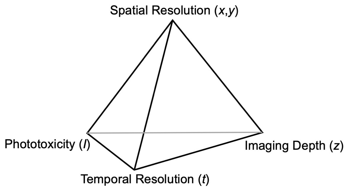
If you want to learn about Betzig’s career and work, watch the video at the bottom of this post. In it, he explains how designing a new microscope requires trade-offs between spatial resolution, temporal resolution, imaging depth, and phototoxicity. Many super-resolution fluorescence microscopes (having extraordinarily high spatial resolution, well beyond the diffraction limit) require intense light sources, which cause bleaching or even destruction of the fluorophore. This phototoxicity arises because the excitation light illuminates the entire sample, although much of it doesn’t contribute to the image (as in a confocal microscope). Moreover, microscopes with high spatial resolution must acquire a huge amount of data to form an image, which makes them too slow to follow the rapid dynamics of a living cell.
Eric Betzig’s explanation of the trade-offs between spatial resolution, temporal resolution, imaging depth, and phototoxicity.
Betzig’s key idea is to trade lower spatial resolution for improved temporal resolution and less phototoxicity, creating an unprecedented tool for imaging structure and function in living cells. The figure below illustrates his light-sheet fluorescence microscope.
A light-sheet fluorescence microscope.
The sample (red) is illuminated by a thin sheet of short-wavelength excitation light (blue). This light excites fluorescent molecules in a thin layer of the sample; the position of the sheet can be varied in the z direction, like in MRI. For each slice, the long-wavelength fluorescent light (green) is imaged in the x and y directions by the microscope with its objective lens.
The advantage of this method is that only those parts of the sample to be imaged are exposed to excitation light, reducing the total exposure and therefore the phototoxicity. The thickness of the light sheet can be adjusted to set the depth resolution. The imaging by the microscope can be done quickly, increasing its temporal resolution.
A disadvantage of this microscope is that the fluorescent light is scattered as it passes through the tissue between the light sheet and the objective. However, the degradation of the image can be reduced with adaptive optics, a technique used by astronomers to compensate for scattering caused by turbulence in the atmosphere.
Listen to Betzig describe his career and research in the hour-and-a-half video below. If you don’t have that much time, or you are more interested in the microscope than in Betzig himself, watch the eight-minute video about recent developments in the Advanced Bioimaging Center at Berkeley. It was produced by Seeker, a media company that makes award-winning videos to explain scientific innovations.
Enjoy!
A 2015 talk by Eric Betzig about imaging life at high spatiotemporal resolution.
This is a two-year elementary college physics course for students majoring in science and engineering. The intention of the writers has been to present elementary physics as far as possible in the way in which it is used by physicists working on the forefront of their field. We have sought to make a course which would vigorously emphasize the foundations of physics. Our specific objectives were to introduce coherently into an elementary curriculum the ideas of special relativity, of quantum physics, and of statistical physics.
The course is intended for any student who has had a physics course in high school. A mathematics course including the calculus should be taken at the same time as this course….
The five volumes of the course as planned will include:
The last volume of the Berkeley Physics Course is devoted to the study of large-scale (i.e., macroscopic) systems consisting of many atoms or molecules: thus it provides an introduction to the subjects of statistical mechanics, kinetic theory, thermodynamics, and heat…My aim has been … to adopt a modern point of view and to show, in as systematic and simple a way as possible, how the basic notions of atomic theory lead to a coherent conceptual framework capable of describing and predicting the properties of macroscopic systems.
I love Reif’s book, in part because of nostalgia: it’s the textbook I used in my undergraduate thermodynamics class at the University of Kansas. His Chapter 4 is similar to IPMB’s Chapter 3, where the concepts of heat transfer, absolute temperature, and entropy are shown to result from how the number of states depends on energy. Boltzmann’s factor is derived, and the two-state magnetic system important in magnetic resonance imaging is analyzed. Reif even has short biographies of famous scientists who worked on thermodynamics—such as Boltzmann, Kelvin, and Joule—which I think of as little blog posts built into the textbook. If you want more detail, Reif also has a larger book about statistical and thermal physics that we also cite in IPMB.
Electricity and Magnetism,
Volume 2 of the Berkeley Physics Course,
by Edward Purcell.
Russ and I sort of cite Edward Purcell’s Volume II of the Berkeley Physics Course. Earlier editions of IPMB cited it, but in the 5th edition we cite the book Electricity and Magnetism by Purcell and Morin (2013). It is nearly equivalent to Volume II, but is an update by an additional author. If you want to gain insight into electricity and magnetism, you should read Purcell.
Preface to Volume II
The subject of this volume of the Berkeley Physics Course is electricity and magnetism. The sequence of topics, in rough outline, is not unusual: electrostatics; steady currents; magnetic field; electromagnetic induction; electric and magnetic polarization in matter. However, our approach is different from the traditional one. The difference is most conspicuous in Chaps. 5 and 6 where, building on the work of Vol. I, we treat the electric and magnetic fields of moving charges as manifestations of relativity and the invariance of electric charge.
I love Purcell’s book, but introducing magnetism as a manifestation of special relativity is not the best way to teach the subject to students of biology and medicine. In IPMB we never adopt this view except in a couple teaser homework problems (8.5 and 8.26).
IPMB doesn’t cite Volumes I, III, or IV of the Berkeley Physics Course. If we did, where in the book would those citations be? Kittel, Knight, and Ruderman’s Volume I covers classical mechanics. They analyze the dynamics of particles in a cyclotron so that we could cite it in Chapter 8 of IPMB, and they describe the harmonic oscillator so we could cite it in our Chapter 10. Crawford’s Volume III on waves could be cited in Chapter 13 of IPMB about sound and ultrasound. Wichmann’s Volume IV on quantum mechanics would fit well in the first part of our Chapter 14 on atoms and light.
Do universities adopt the Berkeley Physics Course textbooks anymore? I doubt it. The series is out-of-date, having been published in the 1960s. The use of cgs rather than SI units makes the books seem old fashioned. The preface says it’s a two-year introduction to physics (five semesters, one semester for each book), while most schools offer a one-year (two-semester) sequence. The books don’t have the flashy color photos so common in modern introductory texts. Nevertheless, if you were introduced to physics through the Berkeley Physics Course, you would have a strong grasp of physics fundamentals, and would have more than enough preparation for a course based on Intermediate Physics for Medicine and Biology.
In his introduction, Mahaffey compares the 20th century invention of nuclear power to the 19th century development of steam-powered trains. Then he writes
In this book we will delve into the history of engineering failures,
the problems of pushing into the unknown, and bad luck in nuclear
research, weapons, and the power industry. When you see it all in one
place, neatly arranged, patterns seem to appear. The hidden, underlying
problems may come into focus. Have we been concentrating all
effort in the wrong place? Can nuclear power be saved from itself,
or will there always be another problem to be solved? Will nuclear
fission and its long-term waste destroy civilization, or will it make
civilization possible?
Some of these disasters you have heard about over and over. Some
you have never heard of. In all of them, there are lessons to be learned,
and sometimes the lessons require multiple examples before the reality
sinks in. In my quest to examine these incidents, I was dismayed to
find that what I thought I knew, what I had learned in the classroom,
read in textbooks, and heard from survivors could be inaccurate. A
certain mythology had taken over in both the public and the professional
perceptions of what really happened. To set the record straight,
or at least straighter than it was, I had to find and study buried and
forgotten original reports and first-hand accounts. With declassification
at the federal level, ever-increasing digitization of old documents,
and improvements in archiving and searching, it is now easier to see
what really happened.
So here, Gentle Reader, is your book of train wrecks, disguised as
something in keeping with our 21st century anxieties. In this age, in
which we strive for better sources of electrical and motive energy, there
exists a deep fear of nuclear power, which makes accounts of its worst
moments of destruction that much more important. The purpose of
this book is not to convince you that nuclear power is unsafe beyond
reason, or that it will lead to the destruction of civilization. On the
contrary, I hope to demonstrate that nuclear power is even safer than
transportation by steam and may be one of the key things that will
allow life on Earth to keep progressing; but please form your own conclusions.
The purpose is to make you aware of the myriad ways that
mankind can screw up a fine idea while trying to implement it. Don’t
be alarmed. This is the raw, sometimes disturbing side of engineering,
about which much of humanity has been kept unaware. You cannot
be harmed by just reading about it.
That story of the latest nuclear catastrophe, the destruction of the
Fukushima Daiichi plant in Japan, will be held until near the end. We
are going to start slowly, with the first known incident of radiation
poisoning. It happened before the discovery of radiation, before the
term was coined, back when we were blissfully ignorant of the invisible
forces of the atomic nucleus.
I’ll share just one accident that highlights some of the issues with reactor safety discussed by Mahaffey. It took place at the Chalk River reactor in Ontario, Canada, about 300 miles northeast of Oakland University, as the crow flies.
I found several parallels between the Chalk River and Chernobyl accidents (readers might want to review my earlier post about Chernobyl before reading on). Both hinged on the design of the reactor, and in particular on the type of moderator used to slow neutrons. Both highlight how human error can overcome the most careful of safety designs. Their main difference is that Chalk River was a minor incident while Chernobyl was a catastrophe.
The Chalk River reactor began as a Canadian-British effort during World War II that operated in parallel to America’s Manhattan Project. It’s development has more in common with the plutonium-producing Hanford Site in Washington state than with the bomb-building laboratory in Los Alamos. After Enrico Fermi and his team built the first nuclear reactor in Chicago using graphite as the moderator, the Canadian-British team decided to explore moderation by heavy water. In 1944 they began to build a low-power experimental reactor along the Chalk River. For safety, the reactor has a scram consisting of heavy cadmium plates that would absorb neutrons and would lower into the reactor if a detector recorded too high of a neutron flux, shutting down nuclear fission. The energy production was controlled by raising and lowering the level of heavy water, which could be pumped into the reactor by pushing a switch. As a safety precaution, the pump would turn off after 10 seconds unless the switch was pushed again. To power up the reactor, the operator had to push the switch over and over.
In the summer of 1950 an accident occurred. Two physicists were going to test a new fuel rod design, so the reactor was shut down. The operator knew he would have to push the heavy water button many times to restart the reactor, so he began early, before the physicists were done installing the rod. Growing tired of repeatedly pushing the button, he shoved a wood chip into the switch so it was stuck on. Then the phone rang, and he was distracted by the call. The reactor went supercritical and the two physicists were doused with gamma radiation until the cadmium plates descended. Fortunately, the plates shut down the reactor before too much damage was done, and the physicists survived. Yet, the accident provides many lessons, including how human error can cause the best laid plans to go awry.
Later, a much larger reactor was built at Chalk River, and Mahaffey tells more horror stories about subsequent accidents, including one that required months of cleanup that was led in part by future President Jimmy Carter.
I didn’t realize how all-or-nothing an atomic reactor is. The nuclear fuel is below a critical mass and inert until it reaches a threshold of criticality, at which point it promptly releases a burst of energy and neutrons. Usually it doesn’t blow up like a bomb, because it typically melts before the chain reaction can reach truly explosive proportions. Mahaffey has all sorts of terrifying tales. One begins with a fissile material such as uranium-235 or plutonium-239 dissolved in water; A technician pores the water from one container to another with a more spherical shape, resulting in a flash of neutrons and gamma rays that deliver a lethal dose of radiation.
After scaring us all to death, Mahaffey ends on an upbeat note.
The dangers of continuing to expand nuclear power will always be there, and there could be another unexpected reactor meltdown tomorrow, but the spectacular events that make a compelling narrative may be behind us now. We have learned from each incident. As long as nuclear engineering can strive for new innovations and learn from its history of accidents and mistakes, the benefits that nuclear power can yield for our economy, society, and yes, environment will come.
Atomic Accidents reminded me of Henry Petroski’s wonderful To Engineer is Human: The Role of Failure in Successful Design. The thesis of both books is that you can learn more by examining how things fail than how things succeed. If you want to understand nuclear engineering, the best way is to study atomic accidents.
Pneumoencephalography was performed
by successively injecting small
volumes of air via lumbar puncture and
then removing small volumes of cerebrospinalfluid with the patient sitting upright and the head flexed... Pneumoencephalography
was used primarily
to determine the presence and extent of
posterior fossa or cerebellopontine angle tumors, pituitary tumors, and intraventricular
masses... It was also used to rule
out the presence of lesions affecting the
cerebrospinal fluid spaces in patients with
possible communicating hydrocephalus or
dementia... After the injection
of a sufficient quantity of air, the patient
was rotated, somersaulted, or placed in a
decubitus position to depict the entire ventricularsystem and subarachnoid spaces.
These patients were often uncomfortable,
developed severe headaches, and became
nauseated or vomited.
The early brain imaging techniques… involved such gruesome activities as injecting air into the spinal canal (pneumoencephalography) and rolling the patient about in a specially devised torture chair. Few patients willingly returned for another one of those examinations!
I later learned that while Elsie was at Crownsville, scientists often conducted research on patients there without consent, including one study titled “Pneumoencephalographic and skull X-ray studies in 100 epileptics.” Pneumoencephalography was a technique developed in 1919 for taking images of the brain, which floats in a sea of liquid. That fluid protects the brain from damage, but makes it very difficult to X-ray, since images taken through fluid are cloudy. Pneumoencephalography involved drilling holes into the skulls of research subjects, draining the fluid surrounding their brains, and pumping air or helium into the skull in place of the fluid to allow crisp X-rays of the brain through the skull. the side effects—crippling headaches, dizziness, seizures, vomiting—lasted until the body naturally refilled the skull with spinal fluid, which usually took two to three months. Because pneumoencephalography could cause permanent brain damage and paralysis, it was abandoned in the 1970s.
The application of physics to medicine and biology isn’t just to diagnose diseases that couldn’t be diagnosed before. It also can help replace barbaric procedures by ones that are more humane.
Viruses are tiny packets of genetic material encased in protein. On
their own they are incapable of metabolism or reproduction,
so some scientists do not even consider them as living organisms.
Yet, they can infect a cell and take control of its
metabolic and reproductive functions. The length scale of
viruses is one-tenth of a micron, or 100 nm.
In response to the current Covid-19 pandemic, today I’ll present a micro-course about virology and suggest ways physics contributes to fighting viral diseases.
I’m sometimes careless about distinguishing between the severe acute respiratory syndrome coronavirus 2 (SARS-CoV-2) and the Covid-19 disease it produces. I’ll try to be more careful today. In this post, I’ll refer to SARS-CoV-2 as “the coronavirus” and let virologists worry about the distinctions between different types of coronaviruses. The “2” at the end of SARS-CoV-2 differentiates it from the similar virus responsible for the 2002 SARS epidemic.
The coronavirus is an average sized virus: about 100 nm in diameter. It is enclosed in a lipid bilayer that contains three transmembrane proteins: membrane, envelope, and spike. The spike proteins are the ones that stick out of the coronavirus and give it a crown-like appearance. They’re also the proteins that are recognized by receptors on the host cell and initiate infection. A drug that would interfere with the binding of the spike protein to a receptor would be a potential Covid-19 therapy. A fourth protein, nucleocapsid, is enclosed inside the lipid bilayer and surrounds the genetic material.
Viruses can encode genetic information using DNA or RNA. The coronavirus uses a single strand of messenger RNA, containing about 30,000 bases. For those who remember the central dogma of molecular biology—DNA is transcribed to messenger RNA, which is translated into protein—will know that the RNA of the coronavirus can be translated using the cell’s protein synsthesis machinery, located mainly in the ribosomes. However, only one protein is translated directly: the RNA-dependent RNA polymerase. This enzymecatalyzes the production of more messenger RNA using the virus’s RNA as a template. It is the primary target for the antiviral drug remdesivir. RNA replication lacks the mechanisms to correct errors that cells use when copying DNA, so it is prone to mutations. Fortunately, the coronavirus doesn’t seem to be mutating too rapidly, which makes the development of a vaccine feasible.
The life cycle of the coronavirus consists of 1) binding of the spike protein to an angiotensin-converting enzyme 2 (ACE2) receptor on the extracellular surface of a target cell, 2) injection of the virus RNA, along with the nucleocapsid protein, into the cell, 3) translation of the RNA-dependent RNA polymerase by the cell’s ribosomes and protein synthesis machinery, 4) production of multiple copies of messenger RNA using the RNA-dependent RNA polymerase, 5) translation of this newly-formed messenger RNA to make all the proteins needed for virus production, 6) assembly of virus particles inside the cell, and 7) release of the virus from an infected cell by a process called exocytosis.
Our body responds to the coronavirus by producing antibodies, Y-shaped proteins about 10 nm in size that can bind specifically to an antigen. Antibodies formed in response to Covid-19 bind with the spike protein on the coronavirus’s surface. The details about how this antibody blocks the binding of the spike protein to the ACE2 receptor in our bodies is not entirely clear yet. Such knowledge could be helpful in designing a Covid-19 vaccine.
How can physics contribute to defeating Covid-19? I see several ways. 1) X-ray diffraction is one method to determine the structure of macromolecules, such as the coronavirus’s spike protein and the RNA-dependent RNA polymerase. 2) An Electron microscope can image the coronavirus and its macromolecules. Viruses are too small to resolve using an optical microscope, but (as discussed in Chapter 14 of IPMB) using the wave properties of electrons we can obtain high-resolution images. 3) Computer simulation could be important for predicting how different molecules making up the coronavirus interact with potential drugs. Such calculations might need to include not only the molecular structure but also the mechanism for how charged molecules interact in body fluids, often represented using the Poisson-Boltzmann equation (see Chapter 9 of IPMB). 4) Mathematical modeling is needed to describe how the coronavirus spreads through the population, and how our immune system responds to viral infection. These models are complex, and require the tools of nonlinear dynamics (learn more in Chapter 10 of IPMB).
Ultimately biologists will defeat Covid-19, but physicists have much to contribute to this battle. Together we will overcome this scourge.
How is physics helping in the war against Covid-19?
We considered the logistic differential equation as a model for population growth. The differential equation assumes that the population changes continuously. For some species each generation is distinct, and a difference equation is a better model of the population than a differential equation. An example might be an insect population where one generation lays eggs and dies, and the next year a new generation emerges. A model that has been used for this case is the logistic difference equation or logistic map
yj+1 = a yj (1 – yj/y∞)
with a > 0 and j the generation number. It can again be cast in dimensionless form by defining xj = yj/y∞:
xj+1 = a xj (1 – xj) .
…[Fig. 10.24 in IPMB] shows the remarkable behavior that results when a is increased to 3.1. The values of xj do not come to equilibrium. Rather, they oscillate about the former equilibrium value, taking on first a larger value and then a smaller value. This is a period-2 cycle. The behavior of the map has undergone period doubling…
The period doubling continues with increasing a. For a > 3.449 there is a cycle of period 4… For a > 3.54409 there is a cycle of period 8. The period doubling continues with periods 2N occurring at more and more closely spaced values of a. When a > 3.569946, for many values of a the behavior is aperiodic, and the values of xj never form a repeating sequence. Remarkably, there are ranges of a in this region for which a repeating sequence again occurs, but they are very narrow. The details of this behavior are found in many texts. In the context of ecology they are reviewed in a classic paper by May (1976).
For a < 3.569946, starting from different initial values x0 leads after a number of iterations to the same set of values for the xj. For values of a larger than this, starting from slightly different values of x0 usually leads to very different values of xj, and the differences become greater and greater for larger values of j… This is an example of chaotic behavior, or deterministic chaos.
So I thought that you could have 1, 2, 4, 8, 16, etc., values of xj, or you could have chaos. I didn’t realize there were other choices. Then I read Gleick’s analysis of James Yorke’s paper “Period Three Implies Chaos.”
He proved that in any one-dimensional system, if a regular cycle of period three ever appears, then the same system will also display regular cycles of every other length, as well as completely chaotic cycles. This was the discovery that came as an “electric shock” to physicists like Freeman Dyson. It was so contrary to intuition. You would think it would be trivial to set up a system that would repeat itself in a period-three oscillation without every producing chaos. Yorke showed that it was impossible.
This sent me scurrying back to IPMB to see if we saw any hint of period-three behavior in the logistic map. Sure enough, Fig. 10.27 shows a narrow range around a = 3.8 with period three. Not entirely believing my eyes, I wrote a program to do the calculation (it’s an easy program to write) and found a period-three cycle. I made a plot using a format similar to Fig. 10.24 in IPMB.
A plot of xj vs. j using the logistic map and a = 3.83, showing how the sequence of values converges to three values of x.
Wow! Period three behavior and chaos; who would have thought they go hand-in-hand.
Two months ago—starting March 16 when the coronavirus pandemic closed down in-person classes at Oakland University, where I teach—I began posting to this blog five times a week, Monday to Friday. My hope is that someone out there who was stuck at home found these posts useful. It’s been a grueling pace, and I worry that the quality of the posts has been slipping lately (see, for example, The Barium Enema). Now that the country is opening back up, I’m returning to my traditional schedule: once a week, on Friday mornings.
Before I go, let me remind you that the website for Intermediate Physics for Medicine and Biology is https://sites.google.com/view/hobbieroth/home. There you can find the errata, a mapping that relates blog posts to sections of IPMB (updated this weekend), instructions and game cards for playing Trivial PursuitIPMB (the perfect game for someone stuck at home because of Covid-19; play it with other students via zoom), and other useful stuff.
One last thing (and it’s a big one). For those of you at institutions of higher education, my understanding is that Springer currently is providing access to IPMB at no cost! Their Covid-19 website states
With the Coronavirus outbreak having an unprecedented impact on education, Springer Nature is launching a global program to support learning and teaching at higher education institutions worldwide. We want to support lecturers, teachers and students during this challenging period and hope that this initiative will go some way to help.
Institutions will be able to access more than 500 key textbooks across Springer Nature’s eBook subject collections for free.
IPMB is on their list of books. The Oakland University library has always had an electronic version of IPMB available to OU students, but now it seems that all universities will have access to it. I’m not sure how you go about taking advantage of the offer, but I suggest you go to https://www.springernature.com/gp/librarians/landing/covid19-library-resources and see if you can figure it out.
I am an emeritus professor of physics at Oakland University, and coauthor of the textbook Intermediate Physics for Medicine and Biology. The purpose of this blog is specifically to support and promote my textbook, and in general to illustrate applications of physics to medicine and biology.


.")