Friday, October 18, 2019

Entry Region and Deviations from Poiseuille Flow

Chapter 1 of Intermediate Physics for Medicine and Biology analyzes viscous flow in a tube, also known as Poiseuille flow. Russ Hobbie and I derive the well-known parabolic distribution of speed: motionless at the wall—the no-slip boundary condition—and maximum at the center. In Section 1.20 we consider departures from the parabolic flow profile.
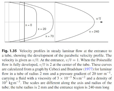
The entry region causes deviations from Poiseuille flow in larger vessels. Suppose that blood flowing with a nearly flat velocity profile enters a vessel, as might happen when blood flowing in a large vessel enters the vessel of interest, which has a smaller radius. At the wall of the smaller vessel, the flow is zero. Since the blood is incompressible, the average velocity is the same at all values of x, the distance along the vessel. (We assume the vessel has a constant cross-sectional area.) However, the velocity profile v(r) changes with distance x along the vessel. At the entrance to the vessel (x = 0), there is a very abrupt velocity change near the walls. As x increases, a parabolic velocity profile is attained. The transition or entry region is shown in Fig. 1.35. In the entry region, the pressure gradient is different from the value for Poiseuille flow. The velocity profile cannot be calculated analytically in the entry region. Various numerical calculations have been made, and the results can be expressed in terms of scaled variables (see, for example, Cebeci and Bradshaw 1977). The Reynolds number used in these calculations was based on the diameter of the pipe, D = 2Rp, and the average velocity. The length of the entry region is

L = 0.05DNR,D = 0.1RpNR,D = 0.2RpNR,Rp.       (1.63)
IPMB’s Figure 1.35 is shown below.

Figure 1.35 from Intermediate Physics for Medicine and Biology.

This figure first appeared in the 3rd edition of IPMB, for which Russ was sole author. I got to wondering how he created it.

Momentum Transfer in Boundary Layers, by Tuncer Cebeci and Peter Bradshaw, superimposed on Intermediate Physics for Medicine and Biology.
Momentum Transfer in
Boundary Layers
,
by Cebeci and Bradshaw.
I checked out the book Momentum Transfer in Boundary Layers, by Cebeci and Bradshaw (1977), through interlibrary loan and found the part about entrance-region flow in their Section 5.7.1. They write
Figures 5.9 and 5.10 show the velocity profiles, u/u0, and the dimensionless centerline (maximum) velocity, uc/u0, as functions of 2x*/Rd in the entrance region of a pipe. Here x* = x/r0 and Rd = u0d/ν. Figure 5.10 also shows the measured values of the centerline velocity obtained by Pfenninger (1951). According to the results of Fig. 5.10, the centerline velocity has almost reached its asymptotic value of 2 at 2x*/Rd = 0.20. Thus the entrance length for a laminar flow in a circular pipe is

le/d = Rd/20       (5.7.12)
Their Fig. 5.9 is

A photograph of Figure 5.9 from Momentum Transfer in Boundary Layers, by Tuncer Cebeci and Peter Bradshaw (1977).
A photograph of Figure 5.9 from Momentum Transfer
in Boundary Layers
, by Cebeci and Bradshaw (1977).
I believe this is the figure Russ used to create his drawing. Clever guy that he is, he seems to have taken the traces, rotated them by 90°, and reflected them across the centerline so they extend from the upper to lower wall. The variable r in their Fig. 5.9 is the distance from the wall, and r0 is the radius of the vessel, so r/r0 = 1 at the center of the vessel and r/r0 = 0 at the wall (don’t ask me why they defined r in this odd way); x* is x/r0, or the distance along the length of the vessel in terms of the vessel radius; ν is the kinematic viscosity, equal to the coefficient of viscosity η divided by the density ρ; and finally Rd is the Reynolds number, defined using the vessel diameter, which Russ and I call NR,D.

At the vessel entrance (x* = 0), the flow is uniform across its cross section with speed u0. The curve corresponding to 2x*/Rd = 0.531 looks almost exactly like Poiseuille flow, with the shape of a parabola and a maximum speed equal to 2u0. For the curve 2x*/Rd = 0.101 the flow is close to, but not exactly, Poiseuille flow. Cebeci and Bradshaw somewhat arbitrarily define the entrance length as corresponding to 2x*/Rd = 0.2.

The example that Russ analyzed in the caption to Fig. 1.35 corresponds to a large vessel such as the brachial artery in your upper arm. A diameter of 4 mm and an entrance length of 240 mm implies a Reynolds number of Rd = 1200. In this case, the entrance length is much greater than the diameter, and is similar to the length of the vessel. If we consider a small vessel like a capillary, however, we get a different picture. A typical Reynolds number for a capillary would be du0ρ/η = (8 × 10⁻⁶ m)(0.001 m/s)(1000 kg/m3)/(3 × 10-3 kg/m/s) = 0.0027, which implies an entrance length of about one nanometer. In other words, the parabolic flow distribution is established almost immediately, over a distance much smaller than the vessel’s length and even its radius. The entrance length is negligible in small vessels like capillaries.

Tuncer Cebeci is a Turkish-American mechanical engineer who worked for the Douglas Aircraft Company and was chair of the Department of Aerospace Engineering at California State University Long Beach. He has authored many textbooks in aeronautics, and developed the Cebeci-Smith model used in computational fluid dynamics. Peter Bradshaw was a professor in the Department of Aeronautics at the Imperial College London and then at Stanford, and is a fellow of the Royal Society. He developed the “Bradshaw Blower,” a type of wind tunnel use to study turbulent boundary layers.

Cebeci and Bradshaw describe why they wrote Momentum Transfer in Boundary Layers in their preface.
This book is intended as an introduction to fluid flows controlled by viscous or turbulent stress gradients and to modern methods of calculating these gradients. It is nominally self-contained, but the explanations of basic concepts are intended as review for senior students who have already taken an introductory course in fluid dynamics, rather than for beginning students. Nearly all stress-dominated flows are shear layers, the most common being the boundary layer on a solid surface. Jets, wakes, and duct flows are also shear layers and are discussed in this volume. Nearly all modern methods of calculating shear layers require the use of digital computers. Computer-based methods, involving calculations beyond the reach of electomechanical desk calculators, began to appear around 10 years ago... With the exception of one or two specialist books... this revolution has not been noticed in academic textbooks, although the new methods are widely used by engineers.
This post illustrates how IPMB merely scratches the surface when explaining how physics impacts medicine and biology. Behind each sentence, each figure, and each reference is a story. I wish Russ and I could tell them all.
Friday, October 11, 2019

A Blog as Ancillary Material for a Physics Textbook

Today I’m attending the Fall 2019 Meeting of the Ohio-Region Section of the American Physical Society and the Michigan Section of the American Association of Physics Teachers, held at Kettering University in Flint, Michigan. Flint is just 45 minutes north of Oakland University, so this is a local meeting for me.

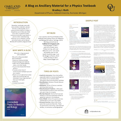
At the meeting I’ll present a poster titled “A Blog as Ancillary Material for a Physics Textbook.” As you can probably guess, the blog I’m referring to is the one you’re reading now. My poster is shown below.

My poster for the Fall 2019 Meeting of the Ohio-Region Section of the American Physical Society and the Michigan Section of the American Association of Physics Teachers.
My poster for the Fall 2019 Meeting of the Ohio-Region Section of the American Physical Society
and the Michigan Section of the American Association of Physics Teachers
The poster begins with my meeting abstract.
Nowadays, textbooks come with many ancillary materials: solution manuals, student guides, etc. A unique ancillary feature is a blog. A blog allows you to keep your book up-to-date, to expand on ideas covered only briefly in your book, to point to other useful learning materials such as websites, articles and other books, and to interact directly with students using your book.
Then I address the question “Why write a blog associated with a textbook?” My reasons are to
  • Keep your book up-to-date. 
  • Present background material. 
  • Offer links to related websites, videos, and other books. 
  • Try out new material for future editions. 
  • Provide a direct line of communication between you and your readers. 
  • Reach out to students from other states and countries who are interested in your topic but don’t have your book (yet). 
  • Have fun. 
  • Increase book sales!
Next I discuss the blog for IPMB.
I am coauthor with Russell Hobbie of the textbook Intermediate Physics for Medicine and Biology (5th edition, Springer, 2015) My blog can be found at hobbieroth.blogspot.com The blog began in 2007. I post once a week, every Friday morning, with over 600 posts so far. I also share the weekly posts on the book’s Facebook page. I use the blogger software, which is free and easy to learn; https://www.blogger.com.
After that, I describe my different types of posts.
  • Useful for Instructors: Posts that will be especially helpful to faculty teaching from your book, such as sample syllabi, information about prerequisites, and links. 
  • Book Reviews: Reviews of books that are related to mine. 
  • Obituaries: Stories of famous scientists who have died recently. 
  • New Homework Problems: I often post new homework problems that instructors can use in class or on exams. 
  • My Own Research: Stories from my own research, to serve as examples of how to apply the material in the textbook. 
  • Lots of Math: Some of my posts are very mathematical, and I warn the reader. 
  • Personal Favorites: About 10% of my posts I list as personal favorites. These are particularly interesting, especially well written, or sometimes autobiographical.
Finally, I provide a sample post. I chose one of my favorites about craps, published on August 10, 2018.

A big thank you to my graduate student Dilmini Wijesinghe, who helped me design the poster. She’ll be at the meeting too, presenting another poster about biomechanics and mechanotransduction. But that’s another story.

Friday, October 4, 2019

Spiral MRI

In Chapter 18 of Intermediate Physics for Medicine and Biology, Russ Hobbie and I discuss a type of magnetic resonance imaging called echo-planar imaging.
In EPI the echoes are not created using π pulses. Instead, they are created by dephasing the spins at different positions along the x axis using a Gx gradient, and then reversing that gradient to rephase the spins, as shown in Fig. 18.32. Whenever the integral of Gx(t) is zero, the spins are all in phase and the signal appears. A large negative Gy pulse sets the initial value of ky to be negative; small positive Gy pulses (“blips”) then increase the value of ky for each successive kx readout. Echo-planar imaging requires strong gradients—at least five times those for normal studies—so that the data can be acquired quickly. Moreover, the rise and fall-times of these pulses are short, which induces large voltages in the coils. Eddy currents are also induced in the patient, and it is necessary to keep these below the threshold for neural activation. These problems can be reduced by using sinusoidally-varying gradient currents. The engineering problems are discussed in Schmitt et al. (1998); in Vlaardingerbroek and den Boer (2004); and in Bernstein et al. (2004).
Echo-Planar Imaging: Theory, Technique and Application, edited by Schmitt, Stehling, and Turner, superimposed on Intermediate Physics for Medicine and Biology.
Echo-Planar Imaging:
Theory, Technique and Application
,
edited by Schmitt, Stehling, and Turner.
To learn more about “sinusoidally-varying gradient currents,” I consulted the first of the three references, Echo-Planar Imaging: Theory, Technique and Application, edited by Franz Schmitt, Michael Stehling, and Robert Turner (Springer, 1998). In his chapter on the “Theory of Echo-Planar Imaging,” Mark Cohen discusses a spiral echo-planar pulse sequence in which the gradient fields have the unusual form Gx = Go t sin(ωt) and Gy = Go t cos(ωt).

Below I show the pulse sequence, which you can compare with the echo-planar imaging sequence in Fig. 18.32 of IPMB if you have the book by your side (don’t you always keep IPMB by your side?). The top two curves are the conventional slice selection sequence: a gradient Gz (red) in the z direction is applied during a radiofrequency π/2 pulse Bx (black), which rotates the spins into the x-y plane. The unconventional readout gradient Gx (blue) varies as an increasing sine wave. It produces a gradient echo at times corresponding approximately to the extrema of the Gx curve (excluding the first small positive peak). The phase encoding gradient Gy (green), an increasing cosine wave, is approximately zero at the echo times, but will shift the phase and therefore impact the amplitude of the echo.
A pulse sequence for spiral echo-planar imaging, based on Fig. 14 of “Theory of Echo-Planar Imaging,” by Mark Cohen in Echo-Planar Imaging: Theory, Technique and Application, edited by Schmitt, Stehling, and Turner.
A pulse sequence for spiral echo-planar imaging,
based on Fig. 14 of “Theory of Echo-Planar Imaging,”
by Mark Cohen.

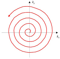
If you look at the output in terms of spatial frequencies (kx, ky), you find that the echos correspond to points along an Archimedean spiral.

The spiral echo-planar imaging technique as viewed in frequency space, based on Fig. 13 of “Theory of Echo-Planar Imaging,” by Mark Cohen, in Echo-Planar Imaging: Theory, Technique and Application, edited by Schmitt, Stehling, and Turner.
The spiral echo-planar imaging technique as viewed in frequency space,
based on Fig. 13 of “Theory of Echo-Planar Imaging,” by Mark Cohen.

Spiral echo-planar imaging has some drawbacks. Data in k-space is not collected over a uniform array, so you need to interpolate onto a square grid before performing a numerical two-dimensional inverse Fourier transform to produce the image. Moreover, you get blurring from chemical shift and susceptibility artifacts. The good news is that you eliminate the rapid turning on and off of gradient pulses, which reduces eddy currents that can cause their own image distortions and possibly neural stimulation. So, spiral imaging has advantages, but the pulse sequence sure looks weird.

Echo-planar imaging in general, and spiral imaging in particular, are very fast. In his chapter on “Spiral Echo-Planar Imaging,” Craig Meyer discusses his philosophy about using EPI.
Spiral scanning is a promising alternative to traditional EPI. The properties of spiral scanning stem from the circularly symmetric nature of the technique. Among the attractive properties of spiral scanning are its efficiency and its good behavior in the presence of flowing material; the most unattractive property is uncorrected inhomogeneity leads to image blurring. Spiral image reconstruction can be performed rapidly using gridding, and there are a number of techniques for compensating for inhomogeneity. There are good techniques for generating efficient spiral gradient waveforms. Among the growing number of applications of spiral scanning are cardiac imaging, angiography, abdominal tumor imaging, functional imaging, and fluoroscopy.

Spiral scanning is a promising technique, but at the present it is still not in routine clinical use. There are many theoretical reasons why spiral scanning may be advantageous for a number of clinical problems, and initial volunteer and clinical studies have yielded very promising results for a number of applications. Still, until spiral scanning is established in routine clinical use, some caution is warranted about proclaiming it to be the answer for any particular question.

Friday, September 27, 2019

The Cauchy Distribution

In an appendix of Intermediate Physics for Medicine and Biology, Russ Hobbie and I analyze the Gaussian probability distribution
An equation for the Gaussian probability distribution.
It has the classic bell shape, centered at mean x with a width determined by the standard deviation σ.

Other distributions have a similar shape. One example is the Cauchy distribution
An equation for the Cauchy probability distribution.
where the distribution is centered at x and has a half-width at half-maximum γ. I initially thought the Cauchy distribution would be as well behaved as any other probability distribution, but it’s not. It has no mean and no standard deviation!

Rather than thinking abstractly about this issue, I prefer to calculate and watch how things fall apart. So, I wrote a simple computer program to generate N random samples using either the Gaussian or the Cauchy distribution. Below is a histogram for each case (N = 1000; Gaussian, x = 0, σ = 1; Cauchy, x = 0, γ = 1).

Histograms for 1000 random samples obtained using the Cauchy (left) and Gaussian (right) probability distribution.

Those samples out on the wings of the Cauchy distribution are what screw things up. The probability falls off so slowly that there is a significant chance of having a random sample that is huge. The histograms shown above are plotted from −20 to 20, but one of the thousand Cauchy samples was about −2400. I’d need to plot the histogram over a range more than one hundred times wider to capture that bin in the histogram. Seven of the samples had a magnitude over one hundred. By contrast, the largest sample from the Gaussian was about 4.6.

What do these few giant samples do to the mean? The average of the thousand samples shown above obtained from the Cauchy distribution is −1.28, which is bigger than the half-width at half-max. The average of the thousand samples obtained from the Gaussian distribution is −0.021, which is much smaller than the standard deviation.

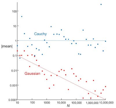
Even more interesting is how the mean varies with N. I tried a bunch of cases, summarized in the figure below.
A plot of the mean versus sample size, for data drawn from the Gassian and Cauchy probability distribution.

There’s a lot of scatter, but the means for the Gaussian data appear to get smaller (closer to the expected value of zero) as N gets larger, The red line is not a fit, but merely drawn by eye. I included it to show how the means fall off with N. It has a slope of −½, implying that the means decay roughly as 1/√N. In contrast, the means for the Cauchy data are large (on the order of one) and don’t fall off with N. No matter how many samples you collect, your mean doesn’t approach the expected value of zero. Some oddball sample comes along and skews the average.

If you calculate the standard deviations for these cases, the problem is even worse. For data generated using the Cauchy distribution, the standard deviation grows with N. For N over a million, the standard deviation is usually over a thousand (remember, the half-width at half-max is one), and for my N = 5,000,000 case the standard deviation was over 600,000. Oddballs dominate the standard deviation.

I’m sorry if my seat-of-the-pants experimental approach to analyzing the Cauchy distribution seems simplistic, but for me it provides insight. The Cauchy distribution is weird, and I’m glad Russ and I didn’t include an appendix about it in Intermediate Physics for Medicine and Biology.

Friday, September 20, 2019

Happy Birthday Professor Fung

Yuan-Cheng Fung celebrated his 100th birthday last Sunday.

Biomechanics: Mechanical Properties of Living Tissues, by Y. C. Fung, superimposed on Intermediate Physics for Medicine and Biology.
Biomechanics: Mechanical
Properties of Living Tissues
,
by Y. C. Fung.
When Russ Hobbie and I needed to cite a general biomechanics textbook in Intermediate Physics for Medicine and Biology, we chose Biomechanics: Mechanical Properties of Living Tissues by “Bert” Fung.
Whenever a force acts on an object, it undergoes a change of shape or deformation. Often these deformations can be ignored… In other cases, such as the contraction of a muscle, the expansion of the lungs, or the propagation of a sound wave, the deformation is central to the problem and must be considered. This book will not develop the properties of deformable bodies extensively; nevertheless, deformable body mechanics is important in many areas of biology (Fung 1993).
According to Google Scholar, Biomechanics has over 10,000 citations, implying it’s a very influential book. In his introduction, Fung writes
Biomechanics seeks to understand the mechanics of living systems. It is an ancient subject and covers a very wide territory. In this book we concentrate on physiology and medical applications, which constitute the majority of recent work in the field. The motivation for research in this area comes from the realization that physiology can no more be understood without biomechanics than an airplane can without aerodynamics. For an airplane, mechanics enables us to design its structure and predict its performance. For an organ, biomechanics helps us to understand its normal function, predict changes due to alterations, and propose methods of artificial intervention. Thus diagnosis, surgery, and prosthesis are closely associated with biomechanics.
A First Course in Continuum Mechanics, by Y. C. Fung, superimposed on Intermediate Physics for Medicine and Biology.
A First Course in
Continuum Mechanics
,
by Y. C. Fung.
Another of Fung’s books that I like is A First Course in Continuum Mechanics. He states his goal in its first sentence. It’s a similar goal to that of IPMB.
Our objective is to learn how to formulate problems in mechanics, and how to reduce vague questions and ideas to precise mathematical statements, as well as to cultivate a habit of questioning, analyzing, designing, and inventing in engineering and science.
A special issue of the Journal of Biomechanical Engineering is dedicated to Fung’s birthday celebration. The editors write
Dr. Fung has been a singular pioneer in the field of Biomechanics, establishing multiple biomechanical theories and paradigms in various organ systems, including the heart, blood vessels, blood cells, and lung... He has mentored and trained many researchers in the biomechanics and bioengineering fields. His books … have become the classic biomechanics textbooks for students and researchers around the world. Dr. Fung is a member of all three U.S. National Academies—National Academy of Sciences, National Academy of Engineering, and National Academy of Medicine. He is also a member of the Chinese Academy of Sciences and a member of Academia Sinica. He has received many awards including the Timoshenko medal, the Russ Prize, and the National Medal of Science.
Fung earned his bachelor’s and master's degrees in aeronautics from the Central University of China in 1941 and 1943. College must have been difficult in China during the Second World War. I bet he has stories to tell. After the war he won a scholarship to come to the United States and study at Caltech, where he earned his PhD in 1948.

Fung joined the faculty at Caltech and remained there for nearly twenty years. In the 1950's, he became interested in biomechanics when his mother was suffering from glaucoma. In 1966, Fung moved to the University of California at San Diego, where he established their bioengineering program. He is known as the “Father of Modern Biomechanics.”

Happy birthday Professor Fung.

 
Yuan-Cheng Fung: 2000 National Medal of Science

2007 Russ Prize video

Friday, September 13, 2019

Intermediate Physics for Medicine and Biology has a New Website

A New Website

This summer I received an email from University Technology Services saying that faculty websites, like the one I maintain about Intermediate Physics for Medicine and Biology, would no longer be supported at Oakland University. In other words, IPMB needed a new online home. So today I announce our new website: https://sites.google.com/view/hobbieroth. If you try to access the old website listed in IPMB, www.oakland.edu/~roth/hobbie, it’ll link you to the new site, but I don’t know how long that will last.

What can you find at our new website? Lots of stuff, including
If you’re looking for my website, it’s changed too, to https://sites.google.com/view/bradroth.

Class Videos

This semester I’m teaching PHY 3250, Biological Physics. I am recording each class, and I’ll upload the videos to YouTube. Anyone can watch the lectures for free, as if it were an online class. I still use the blackboard, and sometimes it’s difficult to read in the video. I hope you can follow most of the lectures.
PHY 3250 class on September 6, 2019, covering biomechanics.


Useful for Instructors

If you scroll down to the box on the right of hobbieroth.blogspot.com you will find a list of labels. Click the one called “Useful for Instructors” and you can find several posts that are….er….useful for instructors. If you’re teaching from IPMB, you might find these posts particularly helpful.

Google Scholar

Below is a screenshot of IPMB’s Google Scholar citation statistics. We’ve averaged 26 citations a year over the last ten years, or one every two weeks. We thank all of you who’ve referenced IPMB. We’re delighted you found it important enough to cite.

A screenshot of the Google Scholar citation data for Intermediate Physics for Medicine and Biology, taken Septeber 1, 2019.

Friday, September 6, 2019

The Linear No-Threshold Model of Radiation Risk

Certain topics discussed in Intermediate Physics for Medicine and Biology always fascinate me. One is the linear no-threshold model. In Section 16.12, Russ Hobbie and I write
In dealing with radiation to the population at large, or to populations of radiation workers, the policy of the various regulatory agencies has been to adopt the linear no-threshold (LNT) model to extrapolate from what is known about the excess risk of cancer at moderately high doses and high dose rates, to low doses, including those below natural background.
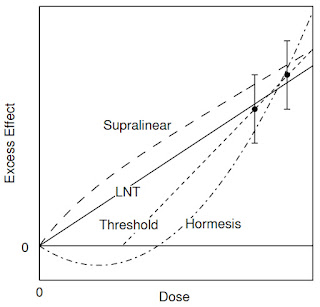
Possible responses to radiation are summarized in Figure 16.51 of IPMB. Scientists continue to debate the LNT model because reliable data (shown by the two data points with their error bars in the upper right) do not extend down to low doses.

Figure 16.51 from Intermediate Physics for Medicine and Biology, showing possible responses to various doses. The two lowest-dose measurements are shown with their error bars.
Figure 16.51 from IPMB, showing possible responses to various doses.
The two lowest-dose measurements are shown with their error bars.
The linear no-threshold assumption is debated in a point/counterpoint article in the August issue of Medical Physics (“The Eventual Rejection of the Linear No-Threshold Theory Will Lead to a Drastic Reduction in the Demand for Diagnostic Medical Physics Services,” Volume 46, Pages 3325-3328). I have discussed before how useful point/counterpoint articles are for teaching medical physics. They provide a glimpse into the controversies that medical physicists grapple with every day. The title of each point/counterpoint article is phrased as a proposition. In this case, Aaron Jones argues for the proposition and Michael O’Connor argues against it. The moderator Habib Zaidi frames the issue in his overview
Controversies about the linear no‐threshold (LNT) hypothesis have been around since the early development of basic concepts in radiation protection and publication of guidelines by professional societies. Historically, this model was conceived over 70 yr ago and is still widely adopted by most of the scientific community and national and international advisory bodies (e.g., International Commission on Radiological Protection, National Council on Radiation Protection and Measurements) for assessing risk from exposure to low‐dose ionizing radiation. The LNT model is currently employed to provide cancer risk estimates subsequent to low level exposures to ionizing radiation despite being criticized as causing unwarranted public fear of all low-dose radiation exposures and costly implementation of unwarranted safety measures. Indeed, linearly extrapolated risk estimates remain hypothetical and have never been rigorously quantified by evidence-based studies. As such, is the LNT model legitimate and its use by regulatory and advisory bodies justified? What would be the impact on our profession if this hypothesis were to be rejected by the scientific community? Would this result in drastic reduction in the demand for diagnostic medical physics services? These questions are addressed in this month’s Point/Counterpoint debate.
Both protagonists give little support to the linear no-threshold hypothesis; they write as if its rejection is inevitable. What is the threshold dose below which risk is negligible? This question is not resolved definitively, but 100 mSv is the number both authors mention.

The linear no-threshold model has little impact for individuals, but is critical for estimating public health risks—such as using backscatter x-ray detectors in airports—when millions of people are exposed to minuscule doses. I’m no expert on this topic so I can’t comment with much authority, but I’ve always been skeptical of the linear no-threshold model.

Much of this point/counterpoint article deals with the impact of the linear no-threshold model on the medical physics job market. I agree with O’Connor that “[The title of the point/counterpoint article] is an interesting proposition as it implies that medical physicists care only about their field and not about whether or not a scientific concept (the LNT) is valid or not,” except “interesting” is not the word I would have chosen. I am skeptical that resolution of the LNT controversy will have a significant consequences for medical physics employment. After we discuss a point/counterpoint article in my PHY 3260 (Medical Physics) class, I insist that students vote either "for" or "against" the proposition. In this case, I agree with O'Connor and vote against it.

I will leave you with O’Connor’s concluding speculation about how rejecting the linear no-threshold model will affect both the population at large and on the future medical physics job market.
In our new enlightened world 30 yr from now, LNT theory has long been discarded, the public are now educated as to the benefits of low doses of ionizing radiation and there is no longer a race to push radiation doses lower and lower in x‐ray imaging. On the contrary, with acceptance of radiation hormesis, a new industry has arisen that offers the public an annual booster dose of radiation every year, particularly if they live in low levels of natural background radiation. How will this booster dose be administered? For those with the means, it might mean an annual trip to the Rocky Mountains. For others it could mean a trip to the nearest clinic for a treatment session with ionizing radiation. Who will oversee the equipment designed to deliver this radiation, to insure that the correct dose is delivered? The medical physicist!

Friday, August 30, 2019

The Book of Why

The Book of Why: The New Science of Cause and Effect, by Judea Pearl and Dana MacKenzie, superimposed on Intermediate Physics for Medicine and Biology.
The Book of Why,
by Judea Pearl.
At Russ Hobbie’s suggestion, I read The Book of Why, by Judea Pearl. This book presents a new way of analyzing data, using causal inferences in addition to more traditional, hypothesis-free statistical methods. In his introduction, Pearl writes
If I could sum up the message of this book in one pithy phrase, it would be that you are smarter than your data. Data do not understand causes and effects; humans do. I hope that the new science of causal inference will enable us to better understand how we do it, because there is no better way to understand ourselves than by emulating ourselves. In the age of computers, this new understanding also brings with it the prospect of amplifying our innate abilities so that we can make better sense of data, be it big or small.
I had a hard time with this book, mainly because I’m not a fan of statistics. Rather than asking “why” questions, I usually ask “what if” questions. In other words, I build mathematical models and then analyze them and make predictions. Intermediate Physics for Medicine and Biology has a similar approach. For instance, what if drift and diffusion both act in a pore; which will dominate under what circumstances (Section 4.12 in IPMB)? What if an ultrasonic wave impinges on an interface between tissues having different acoustic impedances; what fraction of the energy in the wave is reflected (Section 13.3)? What if you divide up a round of radiation therapy into several small fractions; will this preferentially spare healthy tissue (Section 16.9)? Pearl asks a different type of question: the data shows that smokers are more likely to get lung cancer; why? Does smoking cause lung cancer, or is there some confounding effect responsible for the correlation (for instance, some people have a gene that makes them both more susceptible to lung cancer and more likely to smoke)?

Although I can’t say I’ve mastered Pearl’s statistical methods for causal inference, I do like the way he adopts a causal model to test data. Apparently for a long time statisticians analyzed data using no hypotheses, just statistical tests. If they found a correlation, they could not infer causation; does smoking cause lung cancer or does lung cancer cause smoking? Pearl draws many causal diagrams to make his causation assumptions explicit. He then uses these illustrations to derive his statistical model. These drawings remind me of Feynman diagrams that we physicists use to calculate the behavior of elementary particles.

Simpson’s Paradox

Just when my interest in The Book of Why was waning, Pearl shocked me back to attention with Simpson’s paradox.
Imagine a doctor—Dr. Simpson, we’ll call him—reading in his office about a promising new drug (Drug D) that seems to reduce the risk of a heart attack. Excitedly, he looks up the researcher’s data online. His excitement cools a little when he looks at the data on male patients and notices that their risk of a heart attack is actually higher if they take Drug D. “Oh well,” he says, “Drug D must be very effective for women.”

But then he turns to the next table, and his disappointment turns to bafflement. “What is this?” Dr. Simpson exclaims. “It says here that women who took Drug D were also at higher risk of a heart attack. I must be losing my marbles! This drug seems to be bad for women, bad for men, but good for people.”
To illustrate this effect, consider the example analyzed by Pearl. In a clinical trial some patients received a drug (treatment) and some didn’t (control). Patients who subsequently had heart attacks are indicated by red boxes, and patients who did not by blue boxes. In the figure below, the data is analyzed by gender: males and females.

An example of Simpson's paradox, showing men and women being divided into treatment and control groups. Based on The Book of Why, by Judea Pearl and Dana MacKenzie.

One out of twenty (5%) of the females in the control group had heart attacks, while three out of forty (7.5%) in the treatment group did. For women, the drug caused heart attacks! For males, twelve out of forty men in the control group (30%) suffered heart attacks, and eight out of twenty (40%) in the treatment group did. The drug caused heart attacks for the men too!

Now combine the data for men and women.

An example of Simpson's paradox, showing men and women pooled together into treatment and control groups. Based on The Book of Why, by Judea Pearl and Dana MacKenzie.

In the control group, 13 out of 60 patients had a heart attack (22%). In the treatment group, 11 of 60 patients had one (18%). The drug prevented heart attacks! This seems impossible, but if you don’t believe me, count the boxes; it’s not a trick. What do we make of this? As Pearl says “A drug can’t simultaneously cause me and you to have a heart attack and at the same time prevent us both from having heart attacks.”

To resolve the paradox, Pearl notes that this was not a randomized clinical trial. Patients could decide to take the drug or not, and women chose the drug more often then men. The preference for taking the drug is what Pearl calls a “confounder.” The chance of having a heart attack is much greater for men than women, but more women elected to join the treatment group then men. Therefore, the treatment group was overweighted with low-risk women, and the control group was overweighted with high-risk men, so when data was pooled the treatment group looked like they had fewer heart attacks than the control group. In other words, the difference between treatment and control got mixed up with the difference between men and women. Thus, the apparent effectiveness of the drug in the pooled data is a statistical fluke. A random trial would have shown similar data for men and women, but a different result when the data was pooled. The drug causes heart attacks.

Mathematics

The Book of Why contains only a little mathematics; Pearl tries to make the discussion accessible to a wide audience. He does, however, use lots of math in his research. His opinion of math is similar to mine and to IPMB’s.
Many people find formulas daunting, seeing them as a way of concealing rather than revealing information. But to a mathematician, or to a person who is adequately trained in the mathematical way of thinking, exactly the reverse is true. A formula reveals everything: it leaves nothing to doubt or ambiguity. When reading a scientific article, I often catch myself jumping from formula to formula, skipping the words altogether. To me, a formula is a baked idea. Words are ideas in the oven.
One goal of IPMB is to help students gain the skills in mathematical modeling so that formulas reveal rather than conceal information. I often tell my students that formulas aren’t things you stick numbers into to get other numbers. Formulas tell a story. This idea is vitally important. I suspect Pearl would agree.

Modeling

The causal diagrams in The Book of Why aid Pearl in deriving the correct statistical equations needed to analyze data. Toy models in IPMB aid students in deriving the correct differential equations needed to predict behavior. I see modeling as central to both activities: you start with an underlying hypothesis about what causes what, you translate that into mathematics, and then you learn something about your system. As Pearl notes, statistics does not always have this approach.
In certain circles there is an almost religious faith that we can find the answers to these questions in the data itself, if only we are sufficiently clever at data mining. However, readers of this book will know that this hype is likely to be misguided. The questions I have just asked are all causal, and causal questions can never be answered from data alone. They require us to formulate a model of the process that generates the data, or at least some aspects of that process. Anytime you see a paper or a study that analyzes the data in a model-free way, you can be certain that the output of the study will merely summarize, and perhaps transform, but not interpret the data.
I enjoyed The Book of Why, even if I didn’t entirely understand it. It was skillfully written, thanks in part to coauthor Dana MacKenzie. It’s the sort of book that, once finished, I should go back and read again because it has something important to teach me. If I liked statistics more I might do that. But I won’t.

Friday, August 23, 2019

Happy Birthday, Godfrey Hounsfield!

Godfrey Hounsfield (1919-2004).
Godfrey Hounsfield
(1919-2004).
Wednesday, August 28, is the hundredth anniversary of the birth of Godfrey Hounsfield, the inventor of the computed tomography scanner.

In Intermediate Physics for Medicine and Biology, Russ Hobbie and I write
The history of the development of computed tomography is quite interesting (Kalender 2011). The Nobel Prize in Physiology or Medicine was shared in 1979 by a physicist, Allan Cormack, and an engineer, Godfrey Hounsfield…The Nobel Prize acceptance speeches (Cormack 1980; Hounsfield 1980) are interesting to read.
To celebrate the centenary of Hounsfield’s birth, I’ve collected excerpts from his interesting Nobel Prize acceptance speech.
When we consider the capabilities of conventional X-ray methods, three main limitations become obvious. Firstly, it is impossible to display within the framework of a two-dimensional X-ray picture all the information contained in the three-dimensional scene under view. Objects situated in depth, i. e. in the third dimension, superimpose, causing confusion to the viewer.

Secondly, conventional X-rays cannot distinguish between soft tissues. In general, a radiogram differentiates only between bone and air, as in the lungs. Variations in soft tissues such as the liver and pancreas are not discernible at all and certain other organs may be rendered visible only through the use of radio-opaque dyes.

Thirdly, when conventional X-ray methods are used, it is not possible to measure in a quantitative way the separate densities of the individual substances through which the X-ray has passed. The radiogram records the mean absorption by all the various tissues which the X-ray has penetrated. This is of little use for quantitative measurement.

Computed tomography, on the other hand, measures the attenuation of X-ray beams passing through sections of the body from hundreds of different angles, and then, from the evidence of these measurements, a computer is able to reconstruct pictures of the body’s interior...
The technique’s most important feature is its [enormous] sensitivity. It allows soft tissue such as the liver and kidneys to be clearly differentiated, which radiographs cannot do…
It can also very accurately measure the values of X-ray absorption of tissues, thus enabling the nature of tissue to be studied.
These capabilities are of great benefit in the diagnosis of disease, but CT additionally plays a role in the field of therapy by accurately locating, for example, a tumour so indicating the areas of the body to be irradiated and by monitoring the progress of the treatment afterwards...
Famous scientists and engineers often have fascinating childhoods. Learn about Hounsfield’s youth by reading these excerpts from his Nobel biographical statement.
I was born and brought up near a village in Nottinghamshire and in my childhood enjoyed the freedom of the rather isolated country life. After the first world war, my father had bought a small farm, which became a marvellous playground for his five children… At a very early age I became intrigued by all the mechanical and electrical gadgets which even then could be found on a farm; the threshing machines, the binders, the generators. But the period between my eleventh and eighteenth years remains the most vivid in my memory because this was the time of my first attempts at experimentation, which might never have been made had I lived in a city… I constructed electrical recording machines; I made hazardous investigations of the principles of flight, launching myself from the tops of haystacks with a home-made glider; I almost blew myself up during exciting experiments using water-filled tar barrels and acetylene to see how high they could be waterjet propelled…

Aeroplanes interested me and at the outbreak of the second world war I joined the RAF as a volunteer reservist. I took the opportunity of studying the books which the RAF made available for Radio Mechanics and looked forward to an interesting course in Radio. After sitting a trade test I was immediately taken on as a Radar Mechanic Instructor and moved to the then RAF-occupied Royal College of Science in South Kensington and later to Cranwell Radar School. At Cranwell, in my spare time, I sat and passed the City and Guilds examination in Radio Communications. While there I also occupied myself in building large-screen oscilloscope and demonstration equipment as aids to instruction...

It was very fortunate for me that, during this time, my work was appreciated by Air Vice-Marshal Cassidy. He was responsible for my obtaining a grant after the war which enabled me to attend Faraday House Electrical Engineering College in London, where I received a diploma.
I joined the staff of EMI in Middlesex in 1951, where I worked for a while on radar and guided weapons and later ran a small design laboratory. During this time I became particularly interested in computers, which were then in their infancy… Starting in about 1958 I led a design team building the first all-transistor computer to be constructed in Britain, the EMIDEC 1100

I was given the opportunity to go away quietly and think of other areas of research which I thought might be fruitful. One of the suggestions I put forward was connected with automatic pattern recognition and it was while exploring various aspects of pattern recognition and their potential, in 1967, that the idea occurred to me which was eventually to become the EMI-Scanner and the technique of computed tomography...
Happy birthday, Godfrey Hounsfield. Your life and work made a difference.

 Watch “The Scanner Story,” a documentary made by EMI 
about their early computed tomography brain scanners.
The video, filmed in 1978, shows its age but is engaging.

Part Two of “The Scanner Story.”

Friday, August 16, 2019

This View of Life

What’s the biggest idea in science that’s not mentioned in Intermediate Physics for Medicine and Biology? Most of the grand principles of physics appear: quantum mechanics, special relativity, the second law of thermodynamics. The foundations of chemistry are included, such as atomic theory and radioactive decay. Many basic concepts from mathematics are discussed, like calculus and chaos theory. Fundamentals of biology are also present, like the structure of DNA.

In my opinion, the biggest scientific idea never mentioned in Intermediate Physics for Medicine and Biology, not even once, is evolution. As Theodosius Dobzhansky said, “nothing in biology makes sense except in the light of evolution.” So why is evolution absent from IPMB?

A simple, if not altogether satisfactory, answer is that no single book can cover everything. As Russ Hobbie and I write in the preface to IPMB, “This book has become long enough.”

At a deeper level, however, physicists focus on principles that are common to all organisms; which unify our view of life. Evolutionary biologists, on the other hand, delight in explaining how diverse organisms come about through the quirks and accidents of history. Russ and I come from physics, and emphasize unity over diversity.

Ever Since Darwin, by Stephen Jay Gould, superimposed on Intermediate Physics for Medicine and Biology.
Ever Since Darwin,
by Stephen Jay Gould.
Suppose you want to learn more about evolution; how would you do it? I suggest reading books by Stephen Jay Gould (1941-2002), and in particular his collections of essays. I read these years ago and loved them, both for the insights into evolution and for the beauty of the writing. In the prologue of Gould’s first collection—Ever Since Darwin—he says
These essays, written from 1974-1977, originally appeared in my monthly column for Natural History Magazine, entitled “This View of Life.” They range broadly from planetary and geological to social and political history, but they are united (in my mind at least) by the common thread of evolutionary theory—Darwin’s version. I am a tradesman, not a polymath; what I know of planets and politics lies at their intersection with biological evolution.
Is evolution truly missing from Intermediate Physics for Medicine and Biology? Although it’s not discussed explicitly, ideas about how physics constrains evolution are implicit. For instance, one homework problem in Chapter 4 instructs the student to “estimate how large a cell …can be before it is limited by oxygen transport.” Doesn’t this problem really analyze how diffusion impacts natural selection? Another problem in Chapter 3 asks “could a fish be warm blooded and still breathe water [through gills]?” Isn’t this really asking why mammals such as dolphins and whales, which have evolved to live in the water, must nevertheless come to the surface to breathe air? Indeed, many ideas analyzed in IPMB are relevant to evolution.

In Ever Since Darwin, Gould dedicates an essay (Chapter 21, “Size and Shape”) to scaling. Russ and I discuss scaling in Chapter 1 of IPMB. Gould explains that
Animals are physical objects. They are shaped to their advantage by natural selection. Consequently, they must assume forms best adapted to their size. The relative strength of many fundamental forces (gravity, for example) varies with size in a regular way, and animals respond by systematically altering their shapes.
The Panda's Thumb, by Stephen Jay Gould, superimposed on Intermediate Physics for Medicine and Biology.
The Panda's Thumb,
by Stephen Jay Gould.
Gould returns to the topic of scaling in an essay on “Our Allotted Lifetimes,” Chapter 29 in his collection titled The Panda’s Thumb. This chapter contains mathematical expressions (rare in Gould’s essays but common in IPMB) analyzing how breathing rate, heart rate and lifetime scale with size. In his next essay (Chapter 30, “Natural Attraction: Bacteria, the Birds and the Bees”), Gould addresses another topic covered in IPMB: magnetotactic bacteria. He writes
In the standard examples of nature’s beauty—the cheetah running, the gazelle escaping, the eagle soaring, the tuna coursing, and even the snake slithering or the inchworm inching—what we perceive as graceful form also represents an excellent solution to a problem in physics. When we wish to illustrate the concept of adaptation in evolutionary biology, we often try to show that organisms “know” physics—that they have evolved remarkably efficient machines for eating and moving.
Gould knew one of my heroes, Isaac Asimov. In his essay on magnetotactic bacteria, Gould describes how he and Asimov discussed topics similar to those in Edward Purcell’s article “Life at Low Reynolds Number” cited in IPMB.
The world of a bacterium is so unlike our own that we must abandon all our certainties about the way things are and start from scratch. Next time you see Fantastic Voyage... ponder how the miniaturized adventurers would really fare as microscopic objects within a human body... As Isaac Asimov pointed out to me, their ship could not run on its propeller, since blood is too viscous at such a scale. It should have, he said, a flagellum—like a bacterium.
I’m fond of essays, which often provide more insight than journal articles and textbooks. Gould’s 300 essays appeared in every issue of Natural History between 1974 and 2001; he never missed a month. Asimov also had a monthly essay in The Magazine of Fantasy and Science Fiction, and his streak lasted over thirty years, from 1959 to 1992. My twelve-year streak in this blog seems puny compared to these ironmen. Had Gould and Asimov been born a half century later, I wonder if they’d be bloggers?

Gould ends his prologue to The Panda’s Thumb by quoting The Origin of Species, written by his hero Charles Darwin. There in the final paragraph of this landmark book we find a juxtaposition of physics and biology.
Charles Darwin chose to close his great book with a striking comparison that expresses this richness. He contrasted the simpler system of planetary motion, and its result of endless, static cycling, with the complexity of life and its wondrous and unpredictable change through the ages:
There is a grandeur in this view of life, with its several powers, having been originally breathed into a few forms or into one; and that, whilst this planet has gone cycling on according to the fixed law of gravity, from so simple a beginning endless forms most beautiful and most wonderful have been, and are being, evolved.

Listen to Stephen Jay Gould talk about evolution.
https://www.youtube.com/embed/049WuppYa20

 National Public Radio remembers Stephen Jay Gould (May 22, 2002).
https://www.youtube.com/embed/7mTirfwTMsU