The Electric Field Induced During Magnetic Stimulation

Chapter 8 of Intermediate Physics for Medicine and Biology discusses electromagnetic induction and magnetic stimulation of nerves. It doesn't, however, explain how to calculate the electric field. You can learn how to do this from my article “The Electric Field Induced During Magnetic Stimulation” (Electroencephalography and Clinical Neurophysiology, Supplement 43, Pages 268-278, 1991). It begins:

“The Electric Field Induced
During Magnetic Stimulation.”

Magnetic stimulation has been studied widely since its use in 1982 for stimulation of peripheral nerves (Polson et al. 1982), and in 1985 for stimulation of the cortex (Barker et al. 1985). The technique consists of inducing current in the body by Faraday’s law of induction: a time-dependent magnetic field produces an electric field. The transient magnetic field is created by discharging a capacitor through a coil held near the target neuron. Magnetic stimulation has potential clinical applications for the diagnosis of central nervous system disorders such as multiple sclerosis, and for monitoring the corticospinal tract during spinal cord surgery (for review, see Hallett and Cohen 1989). When activating the cortex transcranially, magnetic stimulation is less painful than electrical stimulation.

Appendix 1.

Although there have been many clinical studies of magnetic stimulation, until recently there have been few attempts to measure or calculate the electric field distribution induced in tissue. However, knowledge of the electric field is important for determining where stimulation occurs, how localized the stimulated region is, and what the relative efficacy of different coil designs is. In this paper, the electric field induced in tissue during magnetic stimulation is calculated, and results are presented for stimulation of both the peripheral and central nervous systems.

In Appendix 1 of this article, I derived an expression for the electric field E at position r, starting from

where N is the number of turns in the coil, μ₀ is the permeability of free space (4π × 10^-7 H/m), I is the coil current, r' is the position along the coil, and the integral of dl' is over the coil path. For all but the simplest of coil shapes this integral can't be evaluated analytically, so I used a trick: approximate the coil as a polygon. A twelve-sided polygon looks a lot like a circular coil. You can make the approximation even better by using more sides.

A circular coil (black) approximated by
a 12-sided polygon (red).

With this method I needed to calculate the electric field only from line segments. The calculation for one line segment is summarized in Figure 6 of the paper.

Figure 6 from “The Electric Field
Induced During Magnetic Stimulation.”

I will present the calculation as a new homework problem for IPMB. (Warning: t has two meanings in this problem: it denotes time and is also a dimensionless parameter specifying location along the line segment.)

Section 8.7

Problem 32 ½. Calculate the integral

for a line segment extending from x₂ to x₁. Define δ = x₁ - x₂ and R = r - ½(x₁ + x₂).

(a) Interpret δ and R physically.

(b) Define t as a dimensionless parameter ranging from -½ to ½. Show that r' equals r – R – tδ.

(c) Show that the integral becomes

(d) Evaluate this integral. You may need a table of integrals.

(e) Express the integral in terms of δ, R, and φ (the angle between R and δ).

The resulting expression for the electric field is Equation 15 in the article

Equation (15) in “The Electric Field Induced During Magnetic Stimulation.”

The photograph below shows the preliminary result in my research notebook from when I worked at the National Institutes of Health. I didn't save the reams of scrap paper needed to derive this result.

The November 10, 1988 entry
in my research notebook.

To determine the ends of the line segments, I took an x-ray of a coil and digitized points on it. Below are coordinates for a figure-of-eight coil, often used during magnetic stimulation. The method was low-tech and imprecise, but it worked.

The November 17, 1988 entry
in my research notebook.

Ten comments:

• My coauthors were Leo Cohen and Mark Hallett, two neurologists at NIH. I recommend their four-page paper “Magnetism: A New Method for Stimulation of Nerve and Brain.”
• The calculation above gives the electric field in an unbounded, homogeneous tissue. The article also analyzes the effect of tissue boundaries on the electric field.
• The integral is dimensionless. “For distances from the coil that are similar to the coil size, this integral is approximately equal to one, so a rule of thumb for determining the order of magnitude of E is 0.1 N dI/dt, where dI/dt has units of A/μsec and E is in V/m.”
• The inverse hyperbolic sine can be expressed in terms of logarithms: sinh^-1z = ln[z + √(z² + 1)]. If you're uncomfortable with hyperbolic functions, perhaps logarithms are more to your taste. 
  
• This supplement to Electroencephalography and Clinical Neurophysiology contained papers from the International Motor Evoked Potential Symposium, held in Chicago in August 1989. This excellent meeting guided my subsequent research into magnetic stimulation. The supplement was published as a book: Magnetic Motor Stimulation: Principles and Clinical Experience, edited by Walter Levy, Roger Cracco, Tony Barker, and John Rothwell. 
• Leo Cohen was first author on a clinical paper published in the same supplement: Cohen, Bandinelli, Topka, Fuhr, Roth, and Hallett (1991) “Topographic Maps of Human Motor Cortex in Normal and Pathological Conditions: Mirror Movements, Amputations and Spinal Cord Injuries.”
• To be successful in science you must be in the right place at the right time. I was lucky to arrive at NIH as a young physicist in 1988—soon after magnetic stimulation was invented—and to have two neurologists using the new technique on their patients and looking for a collaborator to calculate electric fields.
• A week after deriving the expression for the electric field, I found a similar expression for the magnetic field. It was never published. Let me know if you need it.
• If you look up my article, please forgive the incorrect units for μ₀ given in the Appendix. They should be Henry/meter, not Farad/meter. In my defense, I had it correct in the body of the article. 
• Correspondence about the article was to be sent to “Bradley J. Roth, Building 13, Room 3W13, National Institutes of Health, Bethesda, MD 20892.” This was my office when I worked at the NIH intramural program between 1988 and 1995. I loved working at NIH as part of the Biomedical Engineering and Instrumentation Program, which consisted of physicists, mathematicians and engineers who collaborated with the medical doctors and biologists. Cohen and Hallett had their laboratory in the NIH Clinical Center (Building 10), and were part of the National Institute of Neurological Disorders and Stroke. Hallett once told me he began his undergraduate education as a physics major, but switched to medicine after one of his professors tried to explain how magnetic fields are related to electric fields in special relativity.

A map of the National Institutes of Health campus
in Bethesda, Maryland.

BrainFacts.org

BrainFacts.org

In this blog, I sometimes share websites related to Intermediate Physics for Medicine and Biology. Recently, I discovered BrainFacts.org.

The human brain is the most complex biological structure in the known universe. Its roughly 86 billion nerve cells power all of our thoughts, perceptions, memories, emotions, and actions. It’s what inspires us to build cities and compels us to gaze at the stars.

That sense of wonder drives BrainFacts.org. We are a public information initiative of The Kavli Foundation, the Gatsby Charitable Foundation, and the Society for Neuroscience – global nonprofit organizations dedicated to advancing brain research.

Powered by the global neuroscience community and overseen by an editorial board of leading neuroscientists from around the world, BrainFacts.org shares the stories of scientific discovery and the knowledge they reveal. Unraveling the mysteries of the brain has the potential to impact every aspect of human experience and civilization.

Join us as we explore the universe between our ears. Because when you know your brain, you know yourself.

“To Understand the Brain,
You Have to Do the Math.”

Browsing BrainFacts.org is an excellent way to learn about neuroscience. The articles are beautifully written, with a professional polish honed by a team of talented science writers (unlike hobbieroth.blogspot.com, written by an aging amateur journalist-wannabe; a one-man-band hawking textbooks). My favorite article—one in the spirit of IPMB—is “To Understand the Brain, You Have to Do the Math” by Alexandre Pouget. He concludes

The brain is the most complex computational device we know in the universe…and unless we do the math, unless we use mathematical theories, there’s absolutely no way we’re ever going to make sense of it.

Browsing BrainFacts.org prompted me to examine how useful Intermediate Physics for Medicine and Biology is for students of neuroscience.

• Chapter 6 is about how nerve axons fire action potentials, which is critical for understanding how neurons in the brain communicate with other neurons and with the rest of the body.
• Chapter 7 discusses functional electrical stimulation of nerves, and mentions deep brain stimulation. It also considers electroencephalography, a tool for monitoring brain function.
• Chapter 8 outlines the physics behind magnetoencephalography as well as transcranial magnetic stimulation.
• Chapter 9 evaluates how weak electric and magnetic fields—say, from power lines or cell phones—affect the brain, and critically assesses if these fields cause brain cancer.
• Chapters 12 and 16 describe tomography, which produces exquisite images of brain anatomy.
• Chapter 17 deals with positron emission tomography, which provides functional information about which regions in the brain are active.
• Chapter 18 analyzes magnetic resonance imaging, including functional MRI and diffusion tensor imaging.

IPMB may not reach the cutting edge of brain science as BrainFacts.org does, but it does discuss many of the technological devices and mathematical tools needed to explore the frontier.

Intermediate Physics for Medicine and Biology plus BrainFacts.org is a winning combination.

 A video about BrainFacts.org by Editor-in-Chief John Morrison

Harry Pennes, Biological Physicist

First page of Pennes (1948) J Appl Physiol 1:93-122.

I admire scientists who straddle the divide between physics and physiology, and who are comfortable with both mathematics and medicine. In particular, I am interested in how such interdisciplinary scientists are trained. Many, like myself, are educated in physics and subsequently shift focus to biology. But more remarkable are those (such as Helmholtz and Einthoven) who begin in biology and later contribute to physics.

Obituary of Harry H. Pennes.

Which brings me to Harry Pennes. Below I reproduce his obituary published in the April 1964 issue of the American Journal of Psychiatry (Volume 120, Page 1030).

Dr. Harry H. Pennes.—Dr. Harry H. Pennes [born 1918], who had been active in clinical work and research in psychiatry and neurology died in November, 1963, at his home in New York City at the age of 45. Dr. Pennes had worked with Dr. Paul H. Hoch and Dr. James Cattell at the Psychiatric Institute of New York Columbia-Presbyterian Medical Center on new techniques of research and medical experimentation.

Dr. Pennes was born in Philadelphia and studied medicine at the University of Pennsylvania where he received a degree in 1942. In 1944 he came to New York to do research at the Neurological Institute. Soon afterward he took a two-year residency at the New York State Psychiatric Institute, and he later joined the staff as Senior Research Psychiatrist. He was also the Research Associate in Psychiatry at Columbia University. At Morris Plains, N. J., Dr. Pennes participated in intensive studies in the Columbia-Greystone Brain Research Project. He did research into chemical warfare from 1953 to 1955 at the Army Chemical Center in Maryland. Later, in Philadelphia, he was Director of Clinical Research for the Eastern Pennsylvania Psychiatric Institute for several years. He subsequently returned to New York a few years ago and resumed private practice.

First page of Wissler (1998).

Before we discuss what’s in his obituary, consider what’s not in it: physics, mathematics, or engineering. Yet, today Pennes is remembered primarily for his landmark contribution to biological physics: the bioheat equation. Russ Hobbie and I analyze this equation in Section 14.11 of Intermediate Physics for Medicine and Biology. In an article titled “Pennes’ 1948 Paper Revisited” (Journal of Applied Physiology, Volume 85, Pages 35-41, 1998), Eugene Wissler wrote:

It can be argued that one of the most influential articles ever published in the Journal of Applied Physiology is the “Analysis of tissue and arterial blood temperatures in the resting human forearm” by Harry H. Pennes, which appeared in Volume 1, No. 2, published in August, 1948. Pennes measured the radial temperature distribution in the forearm by pulling fine thermocouples through the arms of nine recumbent subjects. He also conducted an extensive survey of forearm skin temperature and measured rectal and brachial arterial temperatures. The purpose of Pennes’ study was “to evaluate the applicability of heat flow theory to the forearm in basic terms of the local rate of tissue heat production and volume flow of blood.” An important feature of Pennes’ approach is that his microscopic thermal energy balance for perfused tissue is linear, which means that the equation is amenable to analysis by various methods commonly used to solve the heat-conduction equation. Consequently, it has been adopted by many authors who have developed mathematical models of heat transfer in the human. For example, I used the Pennes equation to analyze digital cooling in 1958 and developed a whole body human thermal model in 1961. The equation proposed by Pennes is now generally known either as the bioheat equation or as the Pennes equation.

So, how did a psychiatrist make a fundamental contribution to physics? I don’t know. Indeed, I have many questions about this fascinating man.

1. Did he work together with a mathematician? No. Pennes was the sole author on the paper. There was no acknowledgment thanking a physicist friend or an engineer buddy. The evidence suggests the work was done by Pennes alone.
2. Did he merely apply an existing model? No. He was the first to include a term in the heat equation to account for convection by flowing blood. He cited a previous study by Gagge et al., but their model was far simpler than his. He didn’t just adopt an existing equation, but rather developed a new and powerful mathematical model. 
3. Was the mathematics elementary? No. He solved the heat equation in cylindrical coordinates. The solution of this partial differential equation included Bessel functions with imaginary arguments (aka modified Bessel functions). He didn’t cite a reference about these functions, but introduced them as if they were obvious.
4. Was his paper entirely theoretical? No. The paper was primarily experimental and the math appeared late in the article when interpreting the results. 
5. Were the experiments easy? No, but they were a little gross. They required threading thermocouples through the arm with no anesthesia. Pennes claimed the “phlegmatic subjects occasionally reported no unusual pain.” I wonder what the nonphlegmatic subjects reported?
6. Was Pennes’s undergraduate degree in physics? I don’t know.
7. Did Pennes’s interest in math arise late in his career? No. His famous 1948 paper was submitted a few weeks before his 30th birthday.
8. Did Pennes work at an institution out of the mainstream that might promote unusual or quirky career paths? No. Pennes worked at Columbia University’s College of Physicians and Surgeons, one of the oldest and most respected medical schools in the country.
9. Did Pennes pick up new skills while in the military? Probably not. He was 23 years old when the Japanese attacked Pearl Harbor, but I can’t find any evidence he served in the military during World War II. He earned his medical degree in 1942 and arrived at Columbia in 1944.  
10. Do other papers published by Pennes suggest an expertise in math? I doubt it. I haven’t read them all, but most study how drugs affect the brain. In fact, his derivation of the bioheat equation seems so out-of-place that I’ve entertained the notion there were two researchers named Harry H. Pennes at Columbia University.
11. Did Pennes’ subsequent career take advantage of his math skills? Again, I am not sure but my guess is no. The Columbia-Greystone Brain Project is famous for demonstrating that lobotomies are not an effective treatment of brain disorders. Research on chemical warfare should require expertise in toxicology. 
12. How did Pennes die? According to Wikipedia he committed suicide. What a tragic loss of a still-young scientist!

I fear my analysis of Harry Pennes provides little insight into how biologists or medical doctors can contribute to physics, mathematics, or engineering. If you know more about Pennes’s life and career, please contact me (roth@oakland.edu).

Even though Harry Pennes’s legacy is the bioheat equation, my guess is that he would’ve been shocked that we now think of him as a biological physicist.

In Vivo Magnetic Recording of Neuronal Activity

In Section 8.9 of Intermediate Physics for Medicine and Biology, Russ Hobbie and I discuss the detection of weak magnetic fields produced by the body.

The detection of weak fields from the body is a technological triumph. The field strength from lung particles is about 10^-9 T [Tesla]; from the heart it is about 10^-10 T; from the brain it is 10^-12 T for spontaneous (α-wave) activity and 10^-13 T for evoked responses. These signals must be compared to 10^-4 T for the earth’s magnetic field. Noise due to spontaneous changes in the earth’s field can be as high as 10^-7 T. Noise due to power lines, machinery, and the like can be 10^-5–10^-4 T.

This triumph was possible because of ultra-sensitive superconducting quantum interference device (SQUID) magnetometers. These magnetometers, however, operate at cryogenic temperatures and therefore must be used outside the body. For instance, to measure the magnetic field of the brain (the magnetoencephalogram), pickup coils must be at least several centimeters from the neurons producing the biomagnetic field because of the thickness of the scalp and skull. A great advantage of SQUIDs is they are completely noninvasive. Yet, when the magnetic field is measured far from the source reconstructing the current distribution is difficult.

Imagine what you could do with a really small magnetometer, say one you could put into the tip of a hypodermic needle. At the cost of being slightly invasive, such a device could measure the magnetic field inside the body right next to its source. The magnetic fields would be larger there and you could get exquisite spatial resolution.

Last September, Laure Caruso and her coworkers published an article about “In Vivo Magnetic Recording of Neuronal Activity” (Neuron, Volume 95, Pages 1283–1291, 2017).

Abstract: Neuronal activity generates ionic flows and thereby both magnetic fields and electric potential differences, i.e., voltages. Voltage measurements are widely used but suffer from isolating and smearing properties of tissue between source and sensor, are blind to ionic flow direction, and reflect the difference between two electrodes, complicating interpretation. Magnetic field measurements could overcome these limitations but have been essentially limited to magnetoencephalography (MEG), using centimeter-sized, helium-cooled extracranial sensors. Here, we report on in vivo magnetic recordings of neuronal activity from visual cortex of cats with magnetrodes , specially developed needle-shaped probes carrying micron-sized, non-cooled magnetic sensors based on spin electronics. Event-related magnetic fields inside the neuropil were on the order of several nanoteslas, informing MEG source models and efforts for magnetic field measurements through MRI. Though the signal-to-noise ratio is still inferior to electrophysiology, this proof of concept demonstrates the potential to exploit the fundamental advantages of magnetophysiology.

A Magnetrode. Adapted from Fig. 1a in Caruso et al. (2017) Neuron 95:1283–1291.

The measurements are made using giant magnetoresistance sensors: a magnetic-field dependent resistor. The size of the sensor was roughly 50 by 50 microns, and was etched to have the shape of a needle with a sharp tip. It can detect magnetic fields of a few nanoTesla (10^-9 T). To test the system, Caruso and her colleagues measured evoked fields in a cat's visual cortex. Remarkably, they performed these experiments with no shielding whatsoever (SQUIDs often require bulky and expensive magnetic shields). When they recorded the magnetic field without averaging it was noisy, so most of their data is after 1000 averages. They removed 50 Hz power line contamination by filtering, and they could distinguish direct magnetic field coupling from capacitive coupling.

When I was in graduate school, John Wikswo and I measured the magnetic field of a single axon using a wire-wound toroidal core. We were able to measure 0.2 nT magnetic fields without averaging and with a signal-to-noise ratio over ten. However, our toroids had a size of a few millimeters, which is larger than Caruso et al.’s magnetrodes. Both methods are invasive, but John and I had to thread the nerve through the toroid, which I think is more invasive than poking the tissue with a needle-like probe.

A couple years ago in this blog, I discussed a way to measure small magnetic fields using optically probed nitrogen-vacancy quantum defects in diamond. That technique has a similar sensitivity as magnetrodes based on giant magnetoresistance, but the recording device is larger and requires an optical readout, which seems to me more complicated than just measuring resistance.

My favorite way to detect fields of the brain would be to use the biomagnetic field as the gradient in magnetic resonance imaging. This method would be completely noninvasive, could be superimposed directly on a traditional magnetic resonance image, and would measure the magnetic field in every pixel simultaneously. Unfortunately, such measurements are barely possible after much averaging even under the most favorable conditions.

Caruso et al. speculate about using implantable magnetrodes with no connecting wires.

Implanted recording probes play an important role in many neurotechnological scenarios. Untethered probes are particularly intriguing, as they avoid connection wires and corresponding limitations.

The recording of tiny biomagnetic fields seems to be undergoing a renaissance, as new detectors are developed. It is truly a technological triumph.

Five New Homework Problems About Diffusion

Diffusion is a central concept in biological physics, but it's seldom taught in physics classes. Russ Hobbie and I cover diffusion in Chapter 4 of Intermediate Physics for Medicine and Biology.

The one-dimensional diffusion equation,

is one of the “big three” partial differential equations. Few analytical solutions to this equation exist. The best known is the decaying Gaussian (Eq. 4.25 in IPMB). Another corresponds to when the concentration is initially constant for negative values of x and is zero for positive values of x (Eq. 4.75). This solution is written in terms of error functions, which are integrals of the Gaussian (Eq. 4.74). I wonder: are there other simple examples illustrating diffusion? Yes!

In this post, my goal is to present several new homework problems that provide a short course in the mathematics of diffusion. Some extend the solutions already included in IPMB, and some illustrate additional solutions. After reading each new problem, stop and try to solve it!

Section 4.13

Problem 48.1. Consider one-dimensional diffusion, starting with an initial concentration of C(x,0)=C_o for x less than 0 and C(x,0)=0 for x greater than 0. The solution is given by Eq. 4.75

where erf is the error function.

(a) Show that for all times the concentration at x=0 is C₀/2.

(b) Derive an expression for the flux density, j = -D ∂C/∂x at x = 0. Plot j as a function of time. Interpret what this equation is saying physically. Note: 

Problem 48.2. Consider one-dimensional diffusion starting with an initial concentration of C(x,0)=C_o for |x| less than L and 0 for |x| greater than L.

(a) Plot C(x,0), analogous to Fig. 4.20.

(b) Show that the solution

obeys both the diffusion equation and the initial condition.

(c) Sketch a plot of C(x,t) versus x for several times, analogous to Fig. 4.22.

(d) Derive an expression for how the concentration at the center changes with time, C(0,t). Plot it.

Problem 48.3. Consider one-dimensional diffusion in the region of x between -L and L. The concentration is zero at the ends, C(±L,t)=0.

(a) If the initial concentration is constant, C(x,0)=C_o, this problem cannot be solved in closed form and requires Fourier series introduced in Chapter 11. However, often such a problem can be simplified using dimensionless variables. Define X = x/L, T = t/(L²/D) and Y = C/C_o. Write the diffusion equation, initial condition, and boundary conditions in terms of these dimensionless variables.

(b) Using these dimensionless variables, consider a different initial concentration Y(X,0)=cos(Xπ/2). This problem has an analytical solution (see Problem 25). Show that Y(X,T)=cos(Xπ/2) e^-π2T/4 obeys the diffusion equation as well as the boundary and initial conditions.

Problem 48.4. In spherical coordinates, the diffusion equation (when the concentration depends only on the radial coordinate r) is (Appendix L)

Let C(r,t) = u(r,t)/r. Determine a partial differential equation governing u(r,t). Explain how you can find solutions in spherical coordinates from solutions of analogous one-dimensional problems in Cartesian coordinates.

Problem 48.5. Consider diffusion in one-dimension from x = 0 to ∞. At the origin the concentration oscillates with angular frequency ω, C(0,t) = C_o sin(ωt).

(a) Determine the value of λ that ensures the expression

obeys the diffusion equation.

(b) Show that the solution in part (a) obeys the boundary condition at x = 0.

(c) Use a trigonometric identity to write the solution as the product of a decaying exponential and a traveling wave (see Section 13.2). Determine the wave speed.

(d) Plot C(x,t) as a function of x at times t = 0, π/2ω, π/ω, 3π/2ω, and 2π/ω.

(e) Describe in words how this solution behaves. How does it change as you increase the frequency?

Of the five problems, my favorite is the last one; be sure to try it. But all the problems provide valuable insight. That’s why we include problems in IPMB, and why you should do them. I have included the solutions to these problems at the bottom of this post (upside down, making it more difficult to check my solutions without you trying to solve the problems first).

Random Walks in Biology,
by Howard Berg.

Interested in learning more about diffusion? I suggest starting with Howard Berg’s book Random Walks in Biology. It is at a level similar to Intermediate Physics for Medicine and Biology.

After you have mastered it, move on to the classic texts by Crank (The Mathematics of Diffusion) and Carslaw and Jaeger (Conduction of Heat in Solids). These books are technical and contain little or no biology. Mathephobes may not care for them. But if you’re trying to solve a tricky diffusion problem, they are the place to go.

Enjoy!

The Mathematics of Diffusion.

The Conduction of Heat in Solids.

I told you these books are technical! (Page 45 of Crank)

Page 4

Page 3

Page 2

Page 1

The Radial Isochron Clock

Section 10.8 of Intermediate Physics for Medicine and Biology describes the radial isochron clock, a toy model for electrical stimulation of nerve or muscle. Russ Hobbie and I write:

Many of the important features of nonlinear systems do not occur with one degree of freedom. We can make a very simple model system that displays the properties of systems with two degrees of freedom by combining the logistic equation for variable r with an angle variable θ that increases at a constant rate:

We can interpret (r,θ) as the polar coordinates of a point in the xy plane. When [time] t has increased from 0 to 1 the angle has increased from 0 to 2π, which is equivalent to starting again with θ = 0. This model system has been used by many authors. Glass and Mackey (1988) have proposed that it be called the radial isochron clock.

Fig. 10.19 of IPMB.

We use this model to analyze phase resetting. Let the clock run until it settles into a stable limit cycle, in which case the signal x(t) is a sinusoidal oscillation. Then apply a stimulus that suddenly increases x by an amount b (see Fig. 10.19 in IPMB) and observe the resulting dynamics. The system returns to its limit cycle, but with a different phase. The first plot in the figure below shows the period T/T₀ of the oscillator just after a stimulus is applied at T_S/T₀; it's the same illustration as in Fig 10.20b of IPMB. Something dramatic appears to be happening at T_S/T₀ = 0.5. What's going on?

The radial isochron clock for different stimulus times and strengths.

The problem with a plot of T/T₀ versus T_S/T₀ is that I have difficulty relating it to the behavior of the signal as a function of time, x(t). Above I plot x versus t for four cases:

• T_S/T₀ = 0.25, b = 0.95 (blue dot). In this case, the stimulus is applied soon after the peak when the signal is decreasing. The sudden jump in x increases the signal so it has further to fall (it must recover lost ground), delaying its descent. As a result is the signal is a behind (is shifted to the right of) the signal that would have been produced had there been no stimulus (red dashed). The figure for b = 1.05 is almost indistinguishable from b = 0.95, so I won’t show it.
• T_S/T₀ = 0.75, b = 0.95 (red dot). The stimulus is applied after the trough when the signal is increasing. The stimulus helps it rise, so it reaches its peak earlier (is shifted to the left) compared to the signal with no stimulus. Again, the figure for b = 1.05 is similar.
• T_S/T₀ = 0.50, b = 0.95 (green dot). When we apply the stimulus near the bottom of the trough, the behavior depends sensitively on stimulus strength b. If b were exactly one and it was applied precisely at the minimum, the result would be x = 0 forever. This would be an unstable equilibrium, like balancing a pencil on its tip. If b was not exactly one, then the key issue is if the signal starts slightly negative (in phase with the unperturbed signal) or slightly positive (out of phase). For b = 0.95, the signal moves to a slightly negative value that corresponds to a trough, meaning that the resulting signal is in phase with the unperturbed signal.
• T_S/T₀ = 0.50, b = 1.05 (yellow dot). If b was a little stronger, then the stimulus moves x to a slightly positive value corresponding to a peak, meaning that the resulting signal is out of phase with the unperturbed signal. Because T/T₀ = 1.5 is equivalent to T/T₀ = 0.5 (the phase just wraps around), the jump of T/T₀ in the top frame does not correspond to a discontinuous physical change.

The drama at T_S/T₀ = 0.5 and b = 1 arises because the stimulus nearly zeros out the signal. The phase of the signal changes from zero to 180 degrees as b changes from less than one to greater than one, but the amplitude of the signal r goes to zero, so the variables x and y change in a continuous way. Some of the homework problems for Section 10.8 in IPMB ask you to explore this on your own. Try them.

The moral of the story is that an abstract illustration—such as Fig. 10.20b in Intermediate Physics for Medicine and Biology—summarizes the behavior of a nonlinear system, but it can’t replace intuition about how the system behaves as a function of time. You need to understand your system “in your gut.” This isn’t true just for the radial isochron clock; it's true for any system. Forget this lesson at your peril!

Anisotropy in Bioelectricity and Biomechanics

Structures: Or Why Things Don't Fall Down,
by James Gordon.

In this third and final post about James Gordon’s book Structures: Or Why Things Don’t Fall Down, I analyze shear.

If tension is about pulling and compression is about pushing, then shear is about sliding. In other words, a shear stress measures the tendency for one part of a solid to slide past the next bit: the sort of thing which happens when you throw a pack of cards on the table or jerk the rug from under someone’s feet. It also nearly always occurs when anything is twisted, such as one’s ankle or the driving shaft of a car…

In Intermediate Physics for Medicine and Biology, Russ Hobbie and I introduce the shear stress, shear strain, and shear modulus, but we don’t do much with them. After Gordon defines these quantities, however, he launches into to a fascinating discussion about shear and anisotropy: different properties in different directions.

Cloth is one of the commonest of all artificial materials and it is highly anisotropic….If you take a square of ordinary cloth in your hands—a handkerchief might do—it is easy to see that the way in which it deforms under a tensile load depends markedly upon the direction in which you pull it. If you pull, fairly precisely, along either the warp or the weft threads, the cloth will extend very little; in other words, it is stiff in tension. Furthermore, in this case, if one looks carefully, one can see that there is not much lateral contraction as a result of the pull…Thus the Poisson’s ratio…is low.

However, if you now pull the cloth at 45° to the direction of the threads—as a dressmaker would say, ‘in the bias direction’—it is much more extensible; that is to say, Young’s modulus in tension is low. This time, though, there is a large lateral contraction, so that, in this direction, the Poisson’s ratio is high.

This analysis led me to ruminate about the different role of anisotropy in bioelectricity versus biomechanics. The mechanical behavior Gordon describes is different than the electrical conductivity of a similar material. As explained in Section 7.9 of IPMB, the current density and electric field in an anisotropic material are related by a conductivity tensor (Eq. 7.39). A cloth-like material would have the same conductivity parallel and perpendicular to the threads, and the off-diagonal terms in the tensor would be zero. Therefore, the conductivity tensor would be proportional to the identity matrix. Homework Problem 26 in Chapter 4 of IPMB shows how to write the tensor in a coordinate system rotated by 45°. The result is that the conductivity is the same in the 45° direction as it is along and across the fibers. As far as its electrical properties are concerned, cloth is isotropic!

I spent much of my career analyzing anisotropy in cardiac muscle, and I was astonished when I realized how different anisotropy appears in mechanics compared to electricity. Gordon’s genius was to analyze a material, such as cloth, that has identical properties in two perpendicular directions, yet is nevertheless mechanically anisotropic. If you study muscle, which has different mechanical and electrical properties along versus across the fibers, the difference between mechanical and electrical anisotropy is not as obvious.

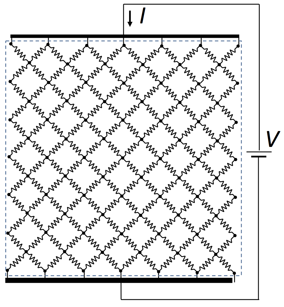
This difference got me thinking: is the electrical conductivity of a cloth-like material really isotropic? Well, yes, it must be when analyzed in terms of the conductivity tensor. But suppose we look at the material microscopically. The figure below shows a square grid of resistors that represents the electrical behavior of tissue. Each resistor is the same, having resistance R. To determine its macroscopic resistance, we apply a voltage difference V and determine the total current I through the grid. The current must pass through N vertical resistors one after the other, so the total resistance through one vertical line is NR. However, there are N parallel lines, reducing the total resistance by a factor of 1/N. The net result: the resistance of the entire grid is the resistance of a single resistor, R.

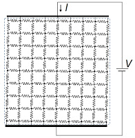
The electrical behavior of tissue represented by a grid of resistors.

Now rotate the grid by 45°. In this case, the current takes a tortuous path through the tissue, with the vertical path length increasing by the square root of two. However, more vertical lines are present per unit length in the horizontal direction (count ’em). How many more? The square root of two more! So, the grid has a resistance R. From a microscopic point of view, the conductivity is indeed isotropic.

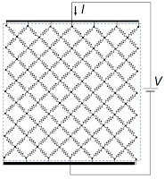
The electrical behavior of tissue represented by a rotated grid of resistors.

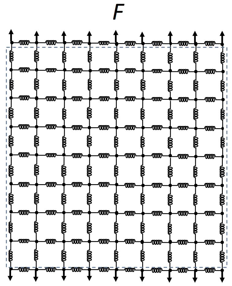
Next, replace the resistors by springs. When you pull upwards, the vertical springs stretch with a spring constant k. Using a similar analysis as performed above, the net spring constant of the grid is also k.

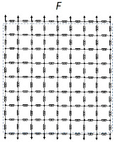
The mechanical behavior of tissue represented by a grid of springs.

Now analyze the grid after it's been rotated by 45°. Even if the spring constant were huge (that is, if the springs were very stiff), the grid would stretch by shearing the rotated squares into diamonds. The tissue would have almost no Young’s modulus in the 45° direction and the Poisson's ratio would be about one; the grid would contract horizontally as it expanded vertically (even if the springs themselves didn't stretch at all). This arises because the springs act as if they're connected by hinges. It reminds me of those gates my wife and I installed to prevent our young daughters from falling down the steps. You would need horizontal struts or vertical ties to prevent such shearing.

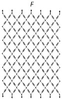
The mechanical behavior of tissue represented by a rotated grid of springs.

In conclusion, you can't represent the mechanical behavior of an isotropic tissue using a square grid of springs without struts or ties. Such a microscopic structure corresponds to cloth, which is anisotropic. A square grid fails to capture properly the shearing of the tissue. You can, however, represent the electrical behavior of an isotropic tissue using a square grid of resistors without “electrical struts or ties.”

Gordon elaborated on the anisotropic mechanical properties of cloth in his own engaging way.

In 1922 a dressmaker called Mlle Vionnet set up shop in Paris and proceeded to invent the “bias cut.” Mlle Vionnet had probably never heard of her distinguished compatriot S. D. Poisson—still less of his ratio—but she realized intuitively that there are more ways of getting a fit than by pulling on strings…if the cloth is disposed at 45°…one can exploit the resulting large lateral contraction so as to get a clinging effect.

Wikipedia adds:

Vionnet's bias cut clothes dominated haute couture in the 1930s, setting trends with her sensual gowns worn by such internationally known actresses as Marlene Dietrich, Katharine Hepburn, Joan Crawford and Greta Garbo. Vionnet’s vision of the female form revolutionized modern clothing, and the success of her unique cuts assured her reputation.

Structures: Or Why Things Don't Fall Down, by J. E. Gordon.

The Pitfalls of Using Handbooks and Formulae

Structures: Or Why Things Don't Fall Down, by J. E. Gordon.

Last week I discussed James Gordon’s book Structures: Or Why Things Don’t Fall Down. The book contains several appendices. The first appendix is ostensibly about using handbooks and formulas to make structural calculations.

Over the last 150 years the theoretical elasticians have analysed the stresses and deflections of structures of almost every conceivable shape when subjected to all sorts and conditions of loads…Fortunately a great deal of this information has been reduced to a set of standard cases or examples the answers to which can be expressed in the form of quite simple formulae.

Then, to my surprise, Gordon changes tack and warns about pitfalls when using these formulas. His counsel, however, applies to all calculations, not just mechanical ones. In fact, his advice is invaluable for any young scientist or engineer. Below, I quote parts of this appendix. Read carefully, and whenever you encounter a word specific to mechanics substitute a general one, or one related to your own field.

[Formulae] must be used with caution.

Appendix 1 of Structures.

1. Make sure that you really understand what the formula is about.
2. Make sure that it really does apply to your particular case.
3. Remember, remember, remember, that these formulae take no account of stress concentrations or other special local conditions.

After this, plug the appropriate loads and dimensions into the formula—making sure that the units are consistent and that the noughts are right. [I’m not sure what “noughts” are, but I think the Englishman Gordon is saying to make sure the decimal point is in the right place.] Then do a little elementary arithmetic and out will drop a figure representing a stress or a deflection.

Now look at this figure with a nasty suspicious eye and think if it looks and feels right. In any case you had better check your arithmetic; are you sure that you haven’t dropped a two?...

If the structure you propose to have made is an important one, the next thing to do, and a very right and proper thing, is to worry about it like blazes. When I was concerned with the introduction of plastic components into aircraft I used to lie awake night after night worrying about them, and I attribute the fact that none of these components ever gave trouble almost entirely to the beneficent effects of worry. It is confidence that causes accidents and worry which prevents them. So go over your sums not once or twice but again and again and again.

Structures: Or Why Things Don't Fall Down.

This is the attitude I try to instill in my students when teaching from Intermediate Physics for Medicine and Biology. I implore them to think before they calculate, and then think again to judge if their answer makes sense. Students sometimes submit an answer to a homework problem (almost always given to five or six significant figures) that is absurd because they didn't look at their answer with a “nasty suspicious eye.” I insist they "remember, remember, remember" the assumptions and limitations of a mathematical model and its resulting formulas. Maybe Gordon goes a little overboard with his “night after night” of lost sleep, but at least he cares enough about his calculation to wonder “again and again and again” if it is correct. A little worry is indeed a “right and proper thing.”

Who would of expected such wisdom tucked away in an appendix about handbooks and formulae?

Structures: Or Why Things Don't Fall Down

Structures: Or Why Things Don't Fall Down,
by James Gordon.

When I was in graduate school, I read a fascinating book by James Gordon titled Structures: Or Why Things Don’t Fall Down. It showed me to how engineers think about mechanics. Recently, I reread Structures and read for the first time its sequel The New Science of Strong Materials: Or Why You Don’t Fall Through the Floor. I enjoyed both books thoroughly.

In Chapter 1 of Intermediate Physics for Medicine and Biology, Russ Hobbie and I discuss two mechanical properties of a material: stiffness and strength. Stiffness describes how much a material lengthens when pulled (that is, strains when stressed), and is quantified by its Young’s modulus. Strength measures how much stress a material can withstand before failing. Gordon summarizes these ideas succinctly.

A biscuit is stiff but weak, steel is stiff and strong, nylon is flexible and strong, raspberry jelly is flexible and weak. The two properties together describe a solid about as well as you can reasonably expect two figures to do.

Just two figures, however, are not sufficient to characterize a material, especially when it's used to build a structure.

The worst sin in an engineering material is not lack of strength or lack of stiffness, desirable as these properties are, but lack of toughness, that is to say, lack of resistance to the propagation of cracks.

Toughness is opposite to brittleness, and is related to but not identical to ductility. It is quantified by the work of fracture—the energy needed to produce a new surface by propagation of a crack through the material—a concept introduced by Alan Griffith during his research on fracture mechanics.

A strained material contains strain energy which would like to be released just as a raised weight contains potential energy and would like to fall…The relief of strain energy …. [is] proportional to the square of the crack length…On the other side of the account book is the surface energy…needed to form the new surfaces and clearly increases as only the first power of the depth of the crack…When the crack is shallow it is consuming more energy as surface energy than it is releasing as relaxed strain energy and therefore conditions are unfavorable for it to propagate. As the crack gets longer however these conditions are reversed and beyond the ‘critical Griffith length’ l_g the crack is producing more energy than it is consuming, so it may start to run away in an explosive manner.

In heterogeneous materials, internal interfaces act as crack stoppers. This makes wood exceptionally tough; Its cellular, fibrous structure prevents a crack from propagating. Toughness is important in biological materials that must undergo large strains without breaking. Wood is not dense (compared to, say, steel), so you get lots of toughness for little weight, which is one reason wood is so popular as a building material. On the other hand, wood isn’t very stiff, and it swells, burns, and rots.

Gordon provides deep insight into the behavior of structures and materials. Consider the stress in the wall of a cylindrical pressure vessel (a long cylinder with spherical end caps). The circumferential stress in the cylinder's wall is given by the Law of Laplace (see IPMB, Chapter 1, Problem 18). The longitudinal stress is equal to the stress in the end caps (the stress in a sphere is two times that in a cylinder, see Problem 19). Thus

the circumferential stress in the wall of a cylindrical pressure vessel is twice the longitudinal stress...One consequence of this must have been observed by everyone who has ever fried a sausage. When the filling inside the sausage swells and the skin bursts, the split is almost always longitudinal.

Then Gordon develops this theme.

Figure 5 from Structures.

If we make a tube or cylinder from such a material [as rubber] and then inflate it, by means of an internal pressure, so as to involve a circumferential strain of 50 per cent or more, then the inflation or swelling process will become unstable, and the tube will bulge out...into a spherical protrusion which a doctor would describe as an “aneurism”....Since veins and arteries do, in fact, generally operate at strains around 50 per cent, and since, as any doctor will tell you, one of the conditions it is most desirable to avoid in blood-vessels is the production of aneurisms, any sort of rubbery elasticity is quite unsuitable....The only sort of elasticity which is completely stable under fluid pressures at high strains is that which is represented by Figure 5 [showing the stress increasing exponentially with the strain]. With minor variations, this shape of stress-strain curve is very common indeed for animal tissue....Materials with this [exponential] type of stress-strain curve are extremely difficult to tear. One reason is, perhaps, that the strain energy stored under such a curve--and therefore available to propagate fracture...is minimized."

He continues

Perhaps partly for these reasons the molecular structure of animal tissue does not often resemble that of rubber or artificial plastics. Most of these natural materials are highly complex, and in many cases they are of a composite nature, with at least two components; that is to say, they have a continuous phase or matrix which is reinforced by means of strong fibres of filaments of another substance. In a good many animals this continuous phase or matrix contains a material called 'elastin', which has a very low modulus and a [flat] stress-strain curve...The elastin is, however, reinforced by an arrangement of bent and zig-zagged fibres of collagen...a protein, very much the same as tendon, which has a high modulus...Because the reinforcing fibres are so much convoluted, when the material is in its resting or low-strain condition they contribute very little to its resistance to extension, and the initial elastic behavior is pretty well that of elastin. However, as the composite tissue stretches the collagen fibres begin to come taut; thus in the extended state the modulus of the material is that of the collagen, which more or less accounts for Figure 5.

As you probably can tell, Gordon writes wonderfully and explains mechanics so it's understandable to a layman. His writing is a model of clarity.

Structures: Or Why Things Don't Fall Down.

Structures was my first exposure to continuum mechanics, but certainly not my last. I was a member of the Mechanical Engineering Section when I worked at the National Institutes of Health, so I was surrounded by outstanding mechanical engineers. My friend Peter Basser—himself a mechanical engineer—would lend me his books, and I recall reading classics such as Love’s A Treatise on the Mathematical Theory of Elasticity and Schlichting’s Boundary Layer Theory. I was impressed by Basser’s model of infusion-induced swelling in the brain and Richard Chadwick’s studies of cardiac biomechanics (Richard was another member of our Mechanical Engineering Section). In many ways, NIH provided a liberal education in physics applied to biology and medicine.

Throughout my career, most of my research has focused on bioelectricity and biomagnetism. Recently, however, I have been working on problems in biomechanics. But that is another story.