Friday, December 16, 2016

Optical Magnetic Detection of Single-Neuron Action Potentials using Quantum Defects in Diamond

A figure from Barry et al., Optical Magnetic Detection of Single-Neuron Action Potentials Using Quantum Defects in Diamond. PNAS, 113:14133–14138, 2016.
A figure from Barry et al., PNAS, 113:14133-14138, 2016.
Last week in this blog, I discussed using a wire-wound toroid to measure the magnetic field of a nerve axon. In the comments to my November 25 post, my friend Raghu Parthasarathy (of the Eighteenth Elephant) pointed me to a recent article by Barry et al.: “Optical magnetic detection of single-neuron action potentials using quantum defects in diamond” (Proceedings of the National Academy of Sciences, 113:14133–14138, 2016). I liked the article, and not just because it cited five of my papers. It presents a new method for measuring biomagnetic fields that does not require toroids or SQUID magnetometers, the only two methods discussed in Chapter 8 of Intermediate Physics for Medicine and Biology.  You can read it online; it’s open access.

Barry et al.’s abstract states:
Magnetic fields from neuronal action potentials (APs) pass largely unperturbed through biological tissue, allowing magnetic measurements of AP dynamics to be performed extracellularly or even outside intact organisms. To date, however, magnetic techniques for sensing neuronal activity have either operated at the macroscale with coarse spatial and/or temporal resolution—e.g., magnetic resonance imaging methods and magnetoencephalography—or been restricted to biophysics studies of excised neurons probed with cryogenic or bulky detectors that do not provide single-neuron spatial resolution and are not scalable to functional networks or intact organisms. Here, we show that AP magnetic sensing can be realized with both single-neuron sensitivity and intact organism applicability using optically probed nitrogen-vacancy (NV) quantum defects in diamond, operated under ambient conditions and with the NV diamond sensor in close proximity (∼10 μm) to the biological sample. We demonstrate this method for excised single neurons from marine worm and squid, and then exterior to intact, optically opaque marine worms for extended periods and with no observed adverse effect on the animal. NV diamond magnetometry is noninvasive and label-free and does not cause photodamage. The method provides precise measurement of AP waveforms from individual neurons, as well as magnetic field correlates of the AP conduction velocity, and directly determines the AP propagation direction through the inherent sensitivity of NVs to the associated AP magnetic field vector.
Here is my poor attempt to explain how their technique works; I must confess I don’t understand it completely. Nitrogen-vacancy defects in a diamond create a spin system that you can use for optically detected electron spin resonance. You shine light onto the system and detect the fluorescence with a photodiode. The shift in the magnetic resonance spectrum contained in the fluoresced light provides a measurement of the magnetic field. For our purposes we can think of the system as a black box that measures the magnetic field; new type of magnetometer.

Barry et al.’s paper started me thinking about the relative advantages and disadvantages of toroids versus optical methods for measuring magnetic fields of nerves.
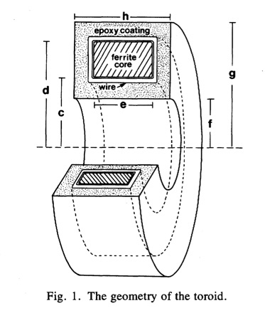
  1. A disadvantage of toroids is that you have to thread the nerve through the toroid center, which usually requires cutting the nerve. My PhD advisor John Wikswo created a “clip-on” toroid that avoids any cutting, but that technique never really caught on. In the optical method, you just drape the nerve over the detector like you would lie down on a bed. Winner: optical method.
  2. The toroid appears to provide a better signal-to-noise ratio than the optical method. Figure 3a in Roth and Wikswo (1985) shows that a signal of about 300 pT peak-to-peak can be detected with a signal-to-noise ratio of roughly 20 with no averaging (I don’t need to look at our 1985 paper to know this, I have a framed copy of this data on display in my office). Figure 2c of Barry et al. (2016) shows a 4000 pT peak-to-peak signal measured optically with a signal-to-noise ratio of about 10 after 600 averages. Perhaps this comparison is unfair because in 1985 we had spent several years optimizing our toroids, whereas this is a first measurement using the optical technique. Nevertheless, I think the toroids have a better signal-to-noise ratio. Winner: toroids.
  3. The optical technique appears to have better spatial resolution, although not dramatically so. Our toroids were typically one or two millimeters in size. In the optical method, the sensing layer is only 13 microns thick, but the length over which the detection occurs is two millimeters, so their method corresponds to a wide but small-diameter toroid. The spatial resolution of both methods could probably be improved, but once the size of the recording device is less than the length over which the action potential upstroke extends (about a millimeter) there is little to be gained by making the detector smaller. Both methods integrate the magnetic signal over the area of the device. Interestingly, the solution to last weeks new homework problem--integrating the biomagnetic field over the cross section of the toroid--is derived in the page 8 of the Barry et al.'s supplementary information. Winner: optical method.
  4. The optical method has better temporal resolution. Both, however, have  temporal resolution adequate to record action potentials with an upstroke of a tenth of a millisecond or longer. The toroid does not record the time course of the magnetic field directly, but rather a mixture of the magnetic field and its derivative, and the technique requires a calibration pulse to get the “frequency compensation” correct. As best I can tell, the optical method measures the magnetic field directly. However, I believe any errors arising from frequency compensation of the toroids are small, and that the temporal resolution of both methods is fine. Winner: optical method.
  5. The toroids are encapsulated in epoxy, so they are biocompatible. I don’t know how biocompatible the optical method is, but I suspect it could be made biocompatible if a thin insulating layer covered the detecting layer, with a very small and probably negligible reduction in spatial resolution. Winner: tie.
  6. The question of convenience is tricky. I am accustomed to using the toroids, so that to me they are not difficult to use, whereas I have never tried the optical method. Nevertheless, I think toroids are more convenient. The optical method requires a static bias magnetic field, and toroids do not. Toroid measurements are insensitive to the exact position of the nerve within the toroid, whereas the optical method appears to be sensitive to the exact placement of the nerve on or near the detector. The optical method requires a spectroscopic analysis of the light signal; the toroid only needs an amplifier to record the current induced in the toroid winding. Finally, the optical method is based on magnetic splitting of spin states and magnetic resonance, whereas toroids rely on good old Faraday induction—my kind of physics. Although I consider toroids more convenient, I would not want to defend that opinion against a skeptical scientist holding a different view, because it is more a matter of taste than science. Winner: toroids.
The result is 3 for the optical method, 2 for toroids, and 1 tie. However, the optical method victories for spatial and temporal resolution were close calls, whereas the toroid victory for signal-to-noise ratio was a landslide. This is not the electoral college: I declare toroids to be the overall winner. (It’s my blog!)

Perhaps a more interesting comparison is for situations where you want to make two-dimensional measurements of current distributions. Barry et al. discuss how the optical method might be extended to do 2D imaging. The traditional method that would be the main competition would be Wikswo’s microSQUID or nanoSQUID: an array of small superconducting coils placed over a sample. But in that case you need cryogenics to keep the coils cold, and I could easily see how a room-temperature array of quantum defect detectors in diamond, recorded optically with a camera, might be simpler.

Both the optical method and toroids require placing a detector near the nerve, so both are invasive. However, if (IF!) the biomagnetic field can be used as the gradient field for magnetic resonance imaging (see my June 3 post) then that technique becomes totally noninvasive. Winner: MRI.

Friday, December 9, 2016

Capabilities of a Toroid-Amplifier System for Magnetic Measurement of Current in Biological Tissue

In Section 8.9 of Intermediate Physics for Medicine and Biology, Russ Hobbie and I discuss the detection of weak magnetic fields.
If the [magnetic] signal is strong enough, it can be detected with conventional coils and signal-averaging techniques that are described in Chap. 11. Barach et al. (1985) used a small detector through which a single axon was threaded. The detector consisted of a toroidal magnetic core wound with many turns of fine wire... Current passing through the hole in the toroid generated a magnetic field that was concentrated in the ferromagnetic material of the toroid. When the field changed, a measurable voltage was induced in the surrounding coil. This neuromagnetic current probe has been used to study many nerve and muscle fibers (Wijesinghe 2010).
I have discussed the neuromagnetic current probe before in this blog. One of the best places to learn more about it is a paper by Frans Gielen, John Wikswo, and me in the IEEE Transactions on Biomedical Engineering (Volume 33, Pages 910–921, 1986). The paper begins
In one-dimensional tissue preparations, bioelectric action currents can be measured by threading the tissue through a wire-wound, ferrite-core toroid that detects the associated biomagnetic field. This technique has several experimental advantages over standard methods used to measure bioelectric potentials. The magnetic measurement does not damage the cell membrane, unlike microelectrode recordings of the internal action potential. Recordings can be made without any electrical contact with the tissue, which eliminates problems associated with the electrochemistry at the electrode-tissue interface. While measurements of the external electric potential depend strongly on the distance between the tissue and the electrode, measurements of the action current are quite insensitive to the position of the tissue in the toroid. Measurements of the action current are also less sensitive to the electrical conductivity of the tissue around the current source than are recordings of the external potential.
Figure 1 of this paper shows the toroid geometry
A illustration of a toroidal coil from Capabilities of a Toroid-Amplifier System for Magnetic Measurement of Current in Biological Tissue, by Gielen et al. (IEEE Trans Biomed Eng, 33:910-921, 1986)
When I was measuring biomagnetic fields back in graduate school, I wanted to relate the magnetic field in the toroid to the current passing through it. For simplicity, assume the current is in a wire passing through the toroid center. The magnetic field B a distance r from a wire carrying current i is (Eq. 8.7 in IPMB)
An equation giving the magnetic field produced by a current-carrying wire.
where μ is the magnetic permeability. The question is, what value should I use for r? Should I use the inner radius, the outer radius, the width, or some combination of these? The answer can be found by solving this new homework problem.
Section 8.2
Problem 11 1/2. Suppose a toroid having inner radius c, outer radius d, and width e is used to detect current i in a wire threading the toroids center. The voltage induced in the toroid is proportional to the magnetic flux through its cross section.
(a) Integrate the magnetic field produced by the current in the wire across the cross section of the ferrite core to obtain the magnetic flux.
(b) Calculate the average magnetic field in the toroid, which is equal to the flux divided by the toroid cross-sectional area.
(c) Define the “effective radius” of the toroid, reff, as the radius needed in Eq. 8.7 to relate the current in the wire to the average magnetic field. Derive an expression for reff in terms of the parameters of the toroid.
(d) If c = 1 mm, d = 2 mm, e = 1 mm, and μ=104μo, calculate reff.
The solution to this homework problem, the effective radius, appears on page 915 of our paper.

Finally, and just for fun, below I reproduce the short bios published with the paper, which appeared 30 years ago.

A brief bio of Frans Gielen, published in IEEE Trans Biomed Eng.

A brief bio of Brad Roth, published in IEEE Trans Biomed Eng.

A brief bio of John Wikswo, published in IEEE Trans Biomed Eng.

Friday, December 2, 2016

The Millikan Oil Drop Experiment

Selected Papers of Great American Physicists, superimposed on Intermediate Physics for Medicine and Biology.
Selected Papers of
Great American Physicists.
When I was in college, I was given a book published by the American Institute of Physics titled Selected Papers of Great American Physicists. Of the seven articles reprinted in this book, my favorite was “On the Elementary Electrical Charge and the Avogadro Constant” by Robert Millikan. Maybe I enjoyed it so much because I had performed the Millikan oil drop experiment as an undergraduate physics major at the University of Kansas. (I have discussed Millikan and his experiment previously in this blog.)

The charge of an electron is encountered often in Intermediate Physics for Medicine and Biology. Its one of those constants thats so fundamental to both physics and biology that its worth knowing how it was first measured. Below is a new homework problem requiring the student to analyze data like that obtained by Millikan. I have designated it for Chapter 6, right after the analysis of the force on a charge in an electric field and the relationship between the electric field and the voltage. I like this problem because it reinforces several concepts already discussed in IPMB (Stoke's law, density, viscosity, electrostatics), it forces the student to analyze data like that obtained experimentally, and it provides a mini history lesson.
Section 6.4

Problem 11 ½. Assume you can measure the time required for a small, charged oil drop to move through air (perhaps by watching it through a microscope with a stop watch in your hand). First, record the time for the drop to fall under the force of gravity. Then record the time for the drop to rise in an electric field. The drop will occasionally gain or lose a few electrons. Assume the drop’s charge is constant over a few minutes, but varies over the hour or two needed to perform the entire experiment, which consists of turning the electric field on and off so one drop goes up and down.

(a) When the drop falls with a constant velocity v1 it is acted on by two forces: gravity and friction given by Stokes’ law. When the drop rises at a constant velocity v2 it is acted on by three forces: gravity, friction, and an electrical force. Derive an expression for the charge q on your drop in terms of v1 and v2. Assume you know the density of the oil ρ, the viscosity of air η, the acceleration of gravity g, and the voltage V you apply across two plates separated by distance L to produce the electric field. These drops, however, are so tiny that you cannot measure their radius a. Therefore, your expression for q should depend on v1, v2, ρ, η, g, V, and L, but not a.
(b) You perform this experiment, and find that whenever the voltage is off the time required for the drop to fall 10 mm is always 12.32 s. Each time you turn the voltage on the drop rises, but the time to rise 10 mm varies because the number of electrons on the drop changes. Successive experiments give rise times of 162.07, 42.31, 83.33, 33.95, 18.96, and 24.33 s. Calculate the charge on the drop in each case. Assume η = 0.000018 Pa s, ρ = 920 kg m-3, V = 5000 V, L = 15 mm, and g = 9.8 m s-2.

(c) Analyze your data to find the greatest common divisor for the charge on the drop, which you can take as the charge of a single electron. Hint: it may be easiest to look at changes in the drops charge over time.
What impressed me most about Millikan’s paper was his careful analysis of sources of systematic error. He went to great pains to determine accurately the viscosity of air, and he accounted for small effects like the mean free path of the air molecules and the drop's buoyancy (effects you can neglect in the problem above). He worried about tiny sources of error such as distortions of the shape of the drop caused by the electric field. When I was a young graduate student, Millikans article provided my model for how you should conduct an experiment.

Friday, November 25, 2016

Intermediate Physicist for Medicine and Biology

In my more contemplative moments, I sometimes ponder: who am I? Or perhaps better: what am I? In my personal life I am many things: son, husband, father, brother, dog-lover, die-hard Cubs fan, Asimov aficionado, Dickens devotee, and mid-twentieth-century-Broadway-musical-theatre admirer.

What I am professionally is not as clear. By training I’m a physicist. Each month I read Physics Today and my favorite publication is the American Journal of Physics. But in many ways I don’t fit well in physics. I don’t understand much of what’s said at our weekly physics colloquium, and I have little or no interest in topics such as high energy physics. Quantum mechanics frightens me.

The term biophysicist doesn’t apply to me, because I don’t work at the microscopic level. I don’t care about protein structures or DNA replication mechanisms. I’m a macroscopic guy.

My work overlaps that of biomedical engineers, and indeed I publish frequently in biomedical engineering journals. But my work is not applied enough for engineering. In the 1990s, when searching desperately for a job, I considered positions in biomedical engineering departments, but I was never sure what I would teach. I have no idea what’s taught in engineering schools. Ultimately I decided that I fit better in a physics department.

Mathematical biologist is a better definition of me. I build mathematical models of biological systems for a living. But I’m at heart neither a mathematician nor a biologist. I find math papers—full of  theorem-proof-theorem-proof—to be tedious. Biologists celebrate life’s diversity, which is exactly the part of biology I like to sweep under the rug.

I’m not a medical physicist. Nothing I have worked on has healed anyone. Besides, medical physicists work in nuclear medicine and radiation therapy departments at hospitals, and they get paid a lot more that I do. No, I’m definitely not a medical physicist. Perhaps one of the most appropriate labels is biological physicist—whatever that means.

Another question is: at what level do I work? I’m not a popularizer of science or a science writer (except when writing this blog, which is more of a hobby; my “Hobbie hobby”). I write research papers and publish them in professional journals. Yet, in these papers I build toy models that are as simple as possible (but no simpler!). Reviewers of my manuscripts write things like “the topic is interesting and the paper is well-written, but the model is too simple; it fails to capture the underlying complexity of the system.” When my simple models grow too complicated, I change direction and work on something else. So my research is neither at an introductory level nor an advanced level.

I guess the best label for me is: Intermediate Physicist for Medicine and Biology.

Friday, November 18, 2016

Molybdenum-99 for Medical Imaging

Molybdenum-99 for Medical Imaging, published by the National Academies Press.
Molybdenum-99 for Medical Imaging,
published by the National Academies Press.
Between 2007 and 2011, I wrote several blog posts about a shortage of the radioisotope technetium-99m (here, here, here, and here). Chapter 17 of Intermediate Physics for Medicine and Biology discusses the many uses of 99mTc in nuclear medicine. It is produced from the decay of molybdenum-99, and shortages arise because of dwindling sources of 99Mo.

Recently, the Committee on State of Molybdenum-99 Production and Utilization and Progress Toward Eliminating Use of Highly Enriched Uranium addressed this issue in their report Molybdenum-99 for Medical Imaging, published by the National Academies Press. Below I reproduce excerpts from the executive summary.
This Academies study was mandated by the American Medical Isotopes Production Act of 2012. Key results for each of the five study charges are summarized below…

Study charge 1: Provide a list of facilities that produce molybdenum-99 (Mo-99) for medical use including an indication of whether these facilities utilize highly enriched uranium (HEU)… About 95 percent of the global supply of Mo-99 for medical use is produced in seven research reactors and supplied from five target processing facilities located in Australia, Canada, Europe, and South Africa. About 5 percent of the global supply is produced in other locations for regional use. About 75 percent of the global supply of Mo-99 for medical use is produced using HEU targets; the remaining 25 percent is produced with low enriched uranium targets….

Study charge 2: Review international production of Mo-99 over the previous 5 years … New Mo-99 suppliers have entered the global supply market since 2009 and further expansions are planned. An organization in Australia (Australian Nuclear Science and Technology Organisation) has become a global supplier and is currently expanding its available supply capacity; existing global suppliers in Europe (Mallinckrodt) and South Africa (NTP Radioisotopes) are also expanding ... A reactor in France (OSIRIS) that produced Mo-99 shut down permanently in December 2015. The reactor in Canada (NRU) will stop the routine production of Mo-99 after October 2016 and permanently shut down at the end of March 2018.

Study charge 3: Assess progress made in the previous 5 years toward establishing domestic production of Mo-99 and associated medical isotopes iodine-131 (I-131) and xenon-133 (Xe-133) … The American Medical Isotopes Production Act of 2012 and financial support from the Department of Energy’s National Nuclear Security Administration … have stimulated private-sector efforts to establish domestic production of Mo-99 and associated medical isotopes. Four NNSA-supported projects and several other private-sector efforts are under way to establish domestic capabilities to produce Mo-99; each project is intended to supply half or more of U.S. needs…. it is unlikely that substantial domestic supplies of Mo-99 will be available before 2018. Neither I-131 nor Xe-133 is currently produced in the United States, but one U.S. organization (University of Missouri Research Reactor Center) is developing the capability to supply I-131; some potential domestic Mo-99 suppliers also have plans to supply I-131 and/or Xe-133 in the future.

Study charge 4: Assess the adequacy of Mo-99 supplies to meet future domestic medical needs, particularly in 2016 and beyond …The United States currently consumes about half of the global supply of Mo-99/technetium-99m (Tc-99m) for medical use; global supplies of Mo-99 are adequate at present to meet domestic needs. Domestic demand for Mo-99/Tc-99m has been declining for at least a decade and has declined by about 25 percent between 2009-2010 and 2014-2015; domestic medical use of Mo-99/Tc-99m is unlikely to increase significantly over the next 5 years. The committee judges that there is a substantial ... likelihood of severe Mo-99/Tc-99m supply shortages after October 2016, when Canada stops supplying Mo-99, lasting at least until current global Mo-99 suppliers complete their planned capacity expansions (planned for 2017) and substantial new domestic Mo-99 supplies enter the market (not likely until 2018 and beyond)….

Study charge 5: Assess progress made by the DOE and others to eliminate worldwide use of HEU in reactor targets and medical isotope production facilities and identify key remaining obstacles for eliminating HEU use… The American Medical Isotopes Production Act of 2012 is accelerating the elimination of worldwide use of HEU for medical isotope production [to reduce the amount of HEU available for production of weapons of mass destruction by terrorist groups]. Current global Mo-99 suppliers have committed to eliminating HEU use in reactor targets and medical isotope production facilities and are making uneven progress toward this goal. Progress is … being impeded by the continued availability of Mo-99 produced with HEU targets … Even after HEU is eliminated from Mo-99 production, large quantities of HEU-bearing wastes from past production will continue to exist at multiple locations throughout the world…
News articles associated with the release of the report can be found here, here, here, and here. The message I get from this report is that the long-term prognosis for 99Mo supplies is promising, but the short-term outlook is worrisome. Let us hope I’m too pessimistic.

Friday, November 11, 2016

Mathematical Physiology

Mathematical Physiology, by James Keener and James Sneyd, with Intermediate Physics for Medicine and Biology.
Mathematical Physiology,
by James Keener and James Sneyd.
In a comment to the blog last week, Frankie mentioned the two-volume textbook Mathematical Physiology (MP), by James Keener and James Sneyd. Russ Hobbie and I cite Keener and Sneyd in Chapter 10 (Feedback and Control) of Intermediate Physics for Medicine and Biology. The Preface to the first edition of MP begins:
It can be argued that of all the biological sciences, physiology is the one in which mathematics has played the greatest role. From the work of Helmholtz and Frank in the last century through to that of Hodgkin, Huxley, and many others in this century [the first edition of MP was published in 1998], physiologists have repeatedly used mathematical methods and models to help their understanding of physiological processes. It might thus be expected that a close connection between applied mathematics and physiology would have developed naturally, but unfortunately, until recently, such has not been the case.

There are always barriers to communication between disciplines. Despite the quantitative nature of their subject, many physiologists seek only verbal descriptions, naming and learning the functions of an incredibly complicated array of components; often the complexity of the problem appears to preclude a mathematical description. Others want to become physicians, and so have little time for mathematics other than to learn about drug dosages, office accounting practices, and malpractice liability. Still others choose to study physiology precisely because thereby they hope not to study more mathematics, and that in itself is a significant benefit. On the other hand, many applied mathematicians are concerned with theoretical results, proving theorems and such, and prefer not to pay attention to real data or the applications of their results. Others hesitate to jump into a new discipline, with all its required background reading and its own history of modeling that must be learned.

But times are changing, and it is rapidly becoming apparent that applied mathematics and physiology have a great deal to offer one another. It is our view that teaching physiology without a mathematical description of the underlying dynamical processes is like teaching planetary motion to physicists without mentioning or using Kepler’s laws; you can observe that there is a full moon every 28 days, but without Kepler’s laws you cannot determine when the next total lunar or solar eclipse will be nor when Halley’s comet will return. Your head will be full of interesting and important facts, but it is difficult to organize those facts unless they are given a quantitative description. Similarly, if applied mathematicians were to ignore physiology, they would be losing the opportunity to study an extremely rich and interesting field of science.

To explain the goals of this book, it is most convenient to begin by emphasizing what this book is not; it is not a physiology book, and neither is it a mathematics book. Any reader who is seriously interested in learning physiology would be well advised to consult an introductory physiology book such as Guyton and Hall (1996) or Berne and Levy (1993), as, indeed, we ourselves have done many times. We give only a brief background for each physiological problem we discuss, certainly not enough to satisfy a real physiologist. Neither is this a book for learning mathematics. Of course, a great deal of mathematics is used throughout, but any reader who is not already familiar with the basic techniques would again be well advised to learn the material elsewhere.

Instead, this book describes work that lies on the border between mathematics and physiology; it describes ways in which mathematics may be used to give insight into physiological questions, and how physiological questions can, in turn, lead to new mathematical problems. In this sense, it is truly an interdisciplinary text, which, we hope, will be appreciated by physiologists interested in theoretical approaches to their subject as well as by mathematicians interested in learning new areas of application.
If you substitute the words “physics” for “mathematics,” “physical” for “mathematical,” and “physicist” for “mathematician,” you would almost think that this preface had been written by Russ Hobbie for an early edition of IPMB.

Many of the topics in MP overlap those in IPMB: diffusion, bioelectricity, osmosis, ion channels, blood flow, and the heart. MP covers additional topics not in IPMB, such as biochemical reactions, calcium dynamics, bursting pancreatic beta cells, and the regulation of gene expression. What IPMB has that MP doesn’t is clinical medical physics: ultrasound, x-rays, tomography, nuclear medicine, and MRI. Both books assume a knowledge of calculus, both average many equations per page, and both have generous collections of homework problems.

Which book should you use? Mathematical Physiology won an award, but Intermediate Physics for Medicine and Biology has an award-winning blog. I’ll take the book with the blog. I bet I know what Frankie will say: “I’ll take both!”

Friday, November 4, 2016

I Spy Physiology

Last year I wrote a blog post about learning biology, aimed at physicists who wanted an introduction to biological ideas. Today, let’s suppose you have completed your introduction to biology. What’s next? Physiology!

What is physiology? Here is the answer provided by the website physiologyinfo.org, sponsored by the American Physiological Society.
Physiology is the study of how the human body works under normal conditions. You use physiology when you exercise, read, breathe, eat, sleep, move or do just about anything.

Physiology is generally divided into ten physiological organ systems: the cardiovascular system, the respiratory system, the immune system, the endocrine system, the digestive system, the nervous system, the renal system, the muscular system, the skeletal system, and the reproductive system.
Screenshot of the I Spy Physiology website.
My favorite part of physiologyinfo.org is the I Spy Physiology blog.
At the American Physiological Society (APS), we believe that physiology is everywhere. It is the foundational science that provides the backbone to our understanding of health and medicine. At its core, physiology is all about understanding the healthy (normal) state of animals—humans included!—what happens when something goes wrong (the abnormal state) and how to get things back to working order. Physiologists study these normal and abnormal states at all levels of the organism: from tiny settings like in a cell to large ones like the whole animal. We also study how humans and animals function, including how they eat, breathe, survive, exercise, heal and sense the environment around them.

On this blog, we’ll endeavor to answer the questions “What is physiology?”, “Where is physiology?”, and “Why does it matter to you?” through current news and health articles and research snippets highlighted by APS members and staff. We’ll also explore the multifaceted world of physiology and follow the path from the lab all the way to the healthy lifestyle recommendations that you receive from your doctor
Other parts of the website I like are “Quizzes and Polls” (I aced the cardiovascular system quiz!) and the podcast library. As a Michigander, I was pleased to see the article about William Beaumont. Finally, I enjoyed Dr. Dolittle’s delightful blog Life Lines, about comparative physiology.

My only complaint about physiologyinfo.org is its lack of physics. That is where Intermediate Physics for Medicine and Biology comes in: IPMB puts the physics in the physiology.

Friday, October 28, 2016

dGEMRIC

dGEMRIC is an acronym for delayed gadolinium enhanced magnetic resonance imaging of cartilage. Adil Bashir and his colleagues provide a clear introduction to dGEMRIC in the abstract of their paper “Nondestructive Imaging of Human Cartilage Glycosaminoglycan Concentration by MRI” (Magnetic Resonance in Medicine, Volume 41, Pages 857–865, 1999).
Despite the compelling need mandated by the prevalence and morbidity of degenerative cartilage diseases, it is extremely difficult to study disease progression and therapeutic efficacy, either in vitro or in vivo (clinically). This is partly because no techniques have been available for nondestructively visualizing the distribution of functionally important macromolecules in living cartilage. Here we describe and validate a technique to image the glycosaminoglycan concentration ([GAG]) of human cartilage nondestructively by magnetic resonance imaging (MRI). The technique is based on the premise that the negatively charged contrast agent gadolinium diethylene triamine pentaacetic acid (Gd(DTPA)2-) will distribute in cartilage in inverse relation to the negatively charged GAG concentration. Nuclear magnetic resonance spectroscopy studies of cartilage explants demonstrated that there was an approximately linear relationship between T1 (in the presence of Gd(DTPA)2-) and [GAG] over a large range of [GAG]. Furthermore, there was a strong agreement between the [GAG] calculated from [Gd(DTPA)2-] and the actual [GAG] determined from the validated methods of calculations from [Na+] and the biochemical DMMB assay. Spatial distributions of GAG were easily observed in T1-weighted and T1-calculated MRI studies of intact human joints, with good histological correlation. Furthermore, in vivo clinical images of T1 in the presence of Gd(DTPA)2- (i.e., GAG distribution) correlated well with the validated ex vivo results after total knee replacement surgery, showing that it is feasible to monitor GAG distribution in vivo. This approach gives us the opportunity to image directly the concentration of GAG, a major and critically important macromolecule in human cartilage.
A schematic illustration of the structure of cartilage.
A schematic illustration of the
structure of cartilage.
The method is based on Donnan equilibrium, which Russ Hobbie and I describe in Section 9.1 of Intermediate Physics for Medicine and Biology. Assume the cartilage tissue (t) is bathed by saline (b). We will ignore all ions except the sodium cation, the chloride anion, and the negatively charged glycosaminoglycan (GAG). Cartilage is not enclosed by a semipermeable membrane, as analyzed in IPMB. Instead, the GAG molecules are fixed and immobile, so they act as if they cannot cross a membrane surrounding the tissue. Both the tissue and bath are electrically neutral, so [Na+]b = [Cl-]b and [Na+]t = [Cl-]t + [GAG-], where we assume GAG is singly charged (we could instead just interpret [GAG-] as being the fixed charge density). At the cartilage surface, sodium and chloride are distributed by a Boltzmann factor: [Na+]t/[Na+]b = [Cl-]b/[Cl-]t = exp(-eV/kT), where V is the electrical potential of the tissue relative to the bath, e is the elementary charge, k is the Boltzmann constant, and T is the absolute temperature. We can solve these equations for [GAG-] in terms of the sodium concentrations: [GAG-] = [Na+]b ( [Na+]t/[Na+]b - [Na+]b/[Na+]t ).

Now, suppose you add a small amount of gadolinium diethylene triamine pentaacetic acid (Gd-DTPA2-); so little that you can ignore it in the equations of neutrality above. The concentrations of Gd-DTPA on the two sides of the articular surface are related by the Boltzmann factor [Gd-DTPA2-]b/[Gd-DTPA2-]t = exp(-2eV/kT) [note the factor of two in the exponent reflecting the valance -2 of Gd-DTPA], implying that [Gd-DTPA2-]b/[Gd-DTPA2-]t = ( [Na+]t/[Na+]b )2. Therefore,

An equation giving the concentration of glycosaminoglycan in cartilage from the measured concentration of gadolinium diethylene triamine pentaacetic acid.

We can determine [GAG-] by measuring the sodium concentration in the bath and the Gd-DTPA concentration in the bath and the tissue. Section 18.6 of IPMB describes how gadolinium shortens the T1 time constant of a magnetic resonance signal, so using T1-weighted magnetic resonance imaging you can determine the gadolinium concentration in both the bath and the tissue.

From my perspective, I like dGEMRIC because it takes two seemingly disparate parts of IPMB, the section of Donnan equilibrium and the section on how relaxation times affect magnetic resonance imaging, and combines them to create an innovative imaging method. Bashir et al.’s paper is eloquent, so I will close this blog post with their own words.
The results of this study have demonstrated that human cartilage GAG concentration can be measured and quantified in vitro in normal and degenerated tissue using magnetic resonance spectroscopy in the presence of the ionic contrast agent Gd(DTPA)2- … These spectroscopic studies therefore demonstrate the quantitative correspondence between tissue T1 in the presence of Gd(DTPA)2- and [GAG] in human cartilage. Applying the same principle in an imaging mode to obtain T1 measured on a spatially localized basis (i.e., T1-calculated images), spatial variations in [GAG] were visualized and quantified in excised intact samples…

In summary, the data presented here demonstrate the validity of the method for imaging GAG concentration in human cartilage… We now have a unique opportunity to study developmental and degenerative disease processes in cartilage and monitor the efficacy of medical and surgical therapeutic measures, for ultimately achieving a greater understanding of cartilage physiology in health and disease.

Friday, October 21, 2016

The Nuts and Bolts of Life: Willem Kolff and the Invention of the Kidney Machine

The Nuts and Bolts of Life: Willem Kolff and the Invention of the Kidney Machine, by Paul Heiney, superimposed on Intermediate Physics for Medicine and BIology.
The Nuts and Bolts of Life:
Willem Kolff and the
Invention of the Kidney Machine,
by Paul Heiney.
In Chapter 5 of Intermediate Physics for Medicine and Biology, Russ Hobbie and I discuss the artificial kidney.
Two compartments, the body fluid and the dialysis fluid, are separated by a membrane that is porous to the small molecules to be removed and impermeable to larger molecules. If such a configuration is maintained long enough, then the concentration of any solute that can pass through the membrane will become the same on both sides.
The history of the artificial kidney is fascinating. Paul Heiney describes this story in his book The Nuts and Bolts of Life: Willem Kolff and the Invention of the Kidney Machine.
Willem Kolff…has battled to mend broken bodies by bringing mechanical solutions to medical problems. He built the first ever artificial kidney and a working artificial heart, and helped create the artificial eye. He s the true founder of the bionic age in which all human parts will be replaceable.
Heiney’s book is not a scholarly treatise and there is little physics in it, but Kolff’s personal story is captivating. Much of the work to develop the artificial kidney was done during World War II, when Kolff’s homeland, the Netherlands, was occupied by the Nazis. Kolff managed to create the first artificial organ while simultaneously caring for his patients, collaborating with the Dutch resistance, and raising five children. Kolff was a tinkerer in the best sense of the word, and his eccentric personality reminds me of the inventor of the implantable pacemaker, Wilson Greatbatch.

Below are some excepts from the first chapter of The Nuts and Bolts of Life. To learn more about Kolff, see his New York Times obituary.
What might a casual visitor have imagined was happening behind the closed door of Room 12a on the first floor of Kampen Hospital in a remote and rural corner of Holland on the night of 11 September 1945? There was little to suggest a small miracle was taking place; in fact, the sounds that emerged from that room could easily have been mistaken for an organized assault.

The sounds themselves were certainly sinister. There was a rumbling that echoed along the tiled corridors of the small hospital and kept patients on the floor below from their sleep; and the sound of what might be a paddle-steamer thrashing through water. All very curious…

The 67-year-old patient lying in Room 12a would have been oblivious to all this. During the previous week she had suffered high fever, jaundice, inflammation of the gall bladder and kidney failure. Not quite comatose, she could just about respond to shouts or the deliberative infliction of pain. Her skin was pale yellow and the tiny amount of urine she produced was dark brown and cloudy….

Before she was wheeled into Room 12a of Kampen Hospital that night, Sofia Schafstadt’s death was a foregone conclusion. There was no cure for her suffering; her kidneys were failing to cleanse her body of the waste it created in the chemical processes of keeping her alive. She was sinking into a body awash in her own poisons….

But that night was to be like no other night in medical history. The young doctor, Willem Kolff, then aged thirty-four and an internist at Kampen Hospital, brought to a great crescendo his work of much of the previous five years. That night, he connected Sofia Schafstadt to his artificial kidney – a machine born out of his own ingenuity. With it, he believed, for the first time ever he could replicate the function of one of the vital organs with a machine working outside the body…

The machine itself was the size of a sideboard and stood by the patient’s bed. The iron frame carried a large enamel tank containing fluid. Inside this rotated a drum around which was wrapped the unlikely sausage skin through which the patient’s blood flowed. And that, in essence, was it: a machine that could undoubtedly be called a contraption was about to become the world’s first successful artificial kidney…

Friday, October 14, 2016

John David Jackson (1925-2016)

Classical Electrodynamics, 3rd Ed, by John David Jackson, superimposed on Intermediate Physics for Medicine and Biology.
Classical Electrodynamics, 3rd Ed,
by John David Jackson.
John David Jackson died on May 20 of this year. I am familiar with Jackson mainly through his book Classical Electrodynamics. Russ Hobbie and I cite Jackson in Chapter 14 of Intermediate Physics for Medicine and Biology.
The classical analog of Compton scattering is Thomson scattering of an electromagnetic wave by a free electron. The electron experiences the electric field E of an incident plane electromagnetic wave and therefore has an acceleration −eE/m. Accelerated charges radiate electromagnetic waves, and the energy radiated in different directions can be calculated, giving Eqs. 15.17 and 15.19. (See, for example, Jackson 1999, Chap. 14.) In the classical limit of low photon energies and momenta, the energy of the recoil electron is negligible.
Classical Electrodynamics, 2nd Ed, by John David Jackson, superimposed on Intermediate Physics for Medicine and Biology.
Classical Electrodynamics, 2nd Ed,
by John David Jackson.
Classical Electrodynamics is usually known simply as “Jackson.” It is one of the top graduate textbooks in electricity and magnetism. When I was a graduate student at Vanderbilt University, I took an electricity and magnetism class based on the second edition of Jackson (the edition with the red cover). My copy of the 2nd edition is so worn that I have its spine held together by tape. Here at Oakland University I have taught from Jackson’s third edition (the blue cover). I remember my shock when I discovered Jackson had adopted SI units in the 3rd edition. He writes in the preface
My tardy adoption of the universally accepted SI system is a recognition that almost all undergraduate physics texts, as well as engineering books at all levels, employ SI units throughout. For many years Ed Purcell and I had a pact to support each other in the use of Gaussian units. Now I have betrayed him!
Classical Electrodynamics, by John David Jackson, editions 2 and 3, with Intermdiate Physics for Medicine and Biology.
Classical Electrodynamics,
by John David Jackson.
Jackson has been my primary reference when I need to solve problems in electricity and magnetism. For instance, I consider my calculation of the magnetic field of a single axon to be little more than a classic “Jackson problem.” Jackson is famous for solving complicated electricity and magnetism problems using the tools of mathematical physics. In Chapter 2 he uses the method of images to calculate the the force between a point charge q and a nearby conducting sphere having the same charge q distributed over its surface. When the distance between the charge and the sphere is large compared to the sphere radius, the repelling force is given by Coulombs law. When the distance is small, however, the charge induces a surface charge of opposite sign on the sphere near it, resulting in an attractive force. Later in Chapter 2, Jackson uses Fourier analysis to calculate the potential inside a two-dimension slot having a voltage V on the bottom surface and grounded on the sides. He finds a series solution, which I think I could have done myself, but then he springs an amazing trick with complex variables in order to sum the series and get an entirely nonintuitive analytical solution involving an inverse tangent of a sine divided by a hyperbolic sine. How lovely.

My favorite is Chapter 3, where Jackson solves Laplace’s equation in spherical and cylindrical coordinate systems. Nerve axons and strands of cardiac muscle are generally cylindrical, so I am a big user of his cylindrical solution based on Bessel functions and Fourier series. Many of my early papers were variations on the theme of solving Laplace’s equation in cylindrical coordinates. In Chapter 5, Jackson analyzes a spherical shell of ferromagnetic material, which is an excellent model for a magnetic shield used in biomagnetic studies.

I have spent most of my career applying what I learned in Jackson to problems in medicine and biology.