The Thermodynamics of the Proton Spin

In Intermediate Physics for Medicine and Biology, Russ Hobbie and I introduce a lot of statistical mechanics and thermodynamics. For instance, in Chapter 3 we describe the Boltzmann factor and the heat capacity, and in Chapter 18 we analyze magnetic resonance imaging by considering the magnetization of the two-state spin system using statistical mechanics. Perhaps we can do a little more.

First, let’s calculate the average energy of a spin-1/2 proton in a magnetic field B. The proton has two states: up and down. Up has the lower energy E_up = -μB, and down has the higher energy E_down = +μB, where μ is the proton’s magnetic moment. Using the Boltzmann factor, the probability of having spin up is P_up = C e^μB/kT, and of spin down is P_down = C e^-μB/kT, where T is the absolute temperature and k is Boltzmann’s constant. The spin must be in one of these two states, so P_up + P_down = 1, or C = 1/(e^μB/kT + e^-μB/kT). The average energy, ⟨E⟩, is P_upE_up + P_downE_down, or

The total energy E of the spin system is just the average energy times the number of spins, E = N⟨E⟩.

Equations are not just things you plug numbers into to get other numbers. Equations tell a physical story. So, whenever I teach the two-state spin system I stress the story, which becomes clearer if we examine the limiting cases of this equation. At high temperatures (μB much less than kT), the argument of the hyperbolic tangent is small, we can use a Taylor expansion for the exponentials, and the average energy is –μ²B²/kT. This is the limit of interest for magnetic resonance imaging, when the average energy increases as the square of the magnetic field. At low temperatures (μB much greater than kT), the argument of the hyperbolic tangent is large, tanh goes to one, and the average energy is –μB. All the spins are in the spin up ground state.

Next, let’s calculate the heat capacity, C = dE/dT. The derivative of the hyperbolic tangent is the hyperbolic secant squared, so

The leading factor is the number of molecules time the Boltzmann constant, which is equal to the number of moles times the gas constant. At high temperatures, C goes to zero because of the leading factor of 1/T². Physically, this result arises because in this case the spins are approximately half spin up and half spin down, so the average energy is about zero, and making the system even hotter won’t change the situation. You typically see this type of behavior in systems that have an upper energy level (as opposed to, say, a system like the harmonic oscillator that has energy levels at increasing energies without bound). At low temperatures, C also goes to zero because the secant goes to zero at large argument. This result arises because the spin down state freezes out: if the system is cold enough no spins can reach the spin down state so the average energy is simply the energy of the spin up ground state.

The heat capacity going to zero as the temperature goes to zero is one way of stating the third law of thermodynamics. Russ and I discuss the first and second laws of thermodynamics in IPMB, but not the third. This is mainly because life occurs at warm temperatures, so the behavior as T approaches absolute zero does not have much biological significance. But although little biology happens around absolute zero, much physics does. To learn more about the world at low temperatures, I recommend the book The Quest for Absolute Zero, by Kurt Mendelssohn. Fascinating reading.

Erythropoietin and Feedback Loops

In Chapter 10 of Intermediate Physics for Medicine and Biology, Russ Hobbie and I discuss feedback loops. We included two new problems about feedback loops in the 5^th edition of IPMB, but as Russ says “you can never have too many examples.” So, here’s another.

The number of red blood cells is controlled by a feedback loop involving the hormone erythropoietin. The higher the erythropoietin concentration, the more red blood cells are produced and therefore the higher the hematocrit. However, the kidney adjusts the production of erythropoietin in response to hypoxia (caused in part by too few red blood cells). The lower the hematocrit the more erythropoietin produced. This new homework problem illustrates the feedback loop. It reinforces concepts from Chapter 10 on feedback and from Chapter 2 on the exponential function, and requires the student to analyze data (albeit made-up data) rather than merely manipulating equations. Warning: the physiological details of this feedback loop are more complicated than discussed in this idealized example.

Section 10.3

Problem 17 ½. Consider a negative feedback loop relating the concentration of red blood cells (the hematocrit, or HCT) to the concentration of the hormone erythropoietin (EPO). In an initial experiment, we infuse blood or plasma intravenously as needed to maintain a constant hematocrit, and measure the EPO concentration. The resulting data are

HCT	EPO
(%)	(mU/ml)
20	200
30	60.1
40	18.1
50	5.45
60	1.64

In a healthy person, the kidney adjusts the concentration of EPO in response to the oxygen concentration (controlled primarily by the hematocrit). In a second experiment, we suppress the kidney’s ability to produce EPO, control the concentration of EPO by infusing the drug intravenously, and measure the resulting hematocrit. We find

EPO	HCT
(mU/ml)	(%)
1	35.0
2	36.0
5	39.1
10	45.0
20	59.5

(a) Plot these results on semilog paper and determine an exponential equation describing each set of data.

(b) Draw a block diagram of the feedback loop, including accurate plots of the two relationships.

(c) Determine the set point (you may have to do this numerically).

(d) Calculate the open loop gain.

Biochemist Eugene Goldwasser first reported purification of erythropoietin when working at the University of Chicago in 1977. In his essay “Erythropoietin: A Somewhat Personal History” he writes about his ultimately successful attempt to isolate erythropoietin from urine samples.

Unfortunately the amounts of active urine concentrates available to us from the NIH source or our own collection were still too small to make significant progress, and it seemed as if purification and characterization of human epo might never be accomplished—that it might remain merely an intriguing biological curiosity. The prospect brightened considerably when Drs. M. Kawakita and T. Miyake instituted a very large-scale collection of urine from patients with aplastic anemia in Kumamato City, Japan. After some lengthy correspondence, Dr. Miyake arrived in Chicago on Christmas Day of 1975, carrying a package representing 2550 liters of urine [!] which he had concentrated using our first-step procedure. He and Charles Kung and I then proceeded systematically to work out a reliable purification method…we eventually obtained about 8 mg of pure human urinary epo .

You can learn more about Goldwasser and his career in his many obituaries, for instance here  and here. A more wide-ranging history of erythropoietin can be found here.

Unequal Anisotropy Ratios

In Chapter 7 of Intermediate Physics for Medicine and Biology, Russ Hobbie and I discuss the bidomain model, a mathematical description of the anisotropic electrical properties of cardiac tissue.

Anisotropy plays an important role in the bidomain model. To see why, consider a solution to Laplace’s equation in a monodomain—a two-dimensional sheet of homogeneous, anisotropic tissue with straight fibers. If the x direction is chosen to be along the fiber direction (the direction of greatest conductivity), then Laplace’s equation becomes

 Now define a new set of coordinates

and

 You can show that in these new coordinates Laplace’s equation becomes

We have removed the effect of anisotropy by rescaling distance in the direction perpendicular to the fibers. If you try a similar trick with the bidomain model … you can find a new coordinate system that removes the effect of anisotropy in either the intracellular space or the extracellular space, but in general you cannot find a coordinate system that removes the anisotropy in both spaces simultaneously (Roth 1992).

My 1992 paper (Journal of Mathematical Biology, Volume 30, Pages 633–646) contains one of my favorite figures, which illustrates the importance of bidomain anisotropy visually. It is equivalent to an old concept from mechanics called the simultaneous diagonalization of two quadratic forms.

Russ and I continue,

Only in the special case of equal anisotropy ratios (σ_ix/σ_iy = σ_ox/σ_oy ) will the equations simplify dramatically. But the anisotropy ratios in the heart are not equal. In the intracellular space the ratio of conductivities parallel and perpendicular to the fibers is about 10:1, while in the extracellular space this ratio is about 4:1 (Roth 1997). Anisotropy plays an essential role in the electrical behavior of the heart, especially during electrical stimulation.

My 1997 paper (IEEE Transactions on Biomedical Engineering, Volume 44, Pages 326–328), published 20 years ago this month, contains an estimate of the bidomain conductivities. After surveying much of the available experimental data, I found

• Intracellular Longitudinal Conductivity     σ_iL     0.2 S/m 
  
• Intracellular Transverse Conductivity        σ_iT     0.02 S/m
• Extracellular Longitudinal Conductivity    σ_eL    0.2 S/m 
• Extracellular Transverse Conductivity       σ_eT    0.08 S/m

This means that the ratio of the conductivity along the fibers to the conductivity across the fibers is 10:1 in the intracellular space, while only 5:2 in the extracellular space.

… Hold on. In IPMB, Russ and I said σ_eL:σ_eT = 4:1, but now I am saying σ_eL:σ_eT = 5:2. Drat! IPMB is wrong. Another entry for the errata…

The 1997 paper is highly cited: Google Scholar lists 178 citations. This perplexes me, because I have many papers that are more significant and innovative, but have far fewer citations. I guess usefulness can sometimes be as important as significance and innovation.

Radiopaedia

A screenshot of Radiopaedia.org.

Readers of Intermediate Physics for Medicine and Biology learn topics in medical physics from a physics point-of-view. Often, however, the discussion in IPMB doesn’t emphasize clinical applications. Where can you get more clinical information? Radiopaedia! Radiopaedia.org is a free online website with a large collection of radiology cases and reference articles.

To see what this site is like, I typed some terms into its search box. When I searched for MRI, I found articles about topics that Russ Hobbie and I present in Chapter 18 of IPMB, such as MRI pulse sequences and MRI artifacts, but also a wealth of clinical topics such as protocols for MRI brain screens, stroke, demyelination, and rectal cancer. The site also contains many case studies of specific patients. And it doesn’t cost a thing.

Radiopaedia has much information about nuclear medicine (Chapter 17 in IPMB). I typed “^99mTc” into the search box and found articles describing a variety of radiopharmaceuticals based on the technetium-99m radioisotope. Also, the site has much information about positron emission tomography (PET) and single photon emission computed tomography (SPECT).

Radiopaedia covers the interaction of x-rays with tissue (Chapter 15 in IPMB) in a variety of articles about different mechanisms such as the photoelectric effect, Compton scattering, and pair-production. Many features of x-ray technology are also discussed (Chapter 16 in IPMB), like x-ray tubes, filters, collimators, grids, and intensifying screens. But also describes x-ray images of specific body parts, such as the abdomen, pelvis, ankle, and shoulder. And all this information is available gratis.

The web site discusses computed tomography qualitatively, but not quantitatively, and lacks much of the mathematics presented in Chapter 12 of IPMB. It contains many medical images, but almost no other figures. For example, the discussion of four generations of CT scanners would benefit from a figure, like Fig. 16.25 in IPMB.

Ultrasound is covered in Chapter 13 of IPMB, and also in Radiopaedia. Topics include transducers, pulse-echo imaging, elastography, and Doppler imaging. Best of all, this valuable information is on the house.

One of the best parts of Radiopaedia is the quiz mode for patient cases. You get to be the doctor, analyzing different medical problems. These cases are too difficult for me to diagnose, but perhaps you can. I find Radiopaedia to be a helpful, no-cost supplement to our book: IPMB supplies the math and physics, while Radiopaedia analyzes the clinical applications.

Did I mention that Radiopaedia is free?

Enjoy.

Top Ten Illustrations in Intermediate Physics for Medicine and Biology

I always love top ten lists, so I prepared a list of my top ten illustrations in Intermediate Physics for Medicine and Biology. These are a subjective, personal selections; you may prefer others. I excluded any figure that was reproduced in IPMB from another publication, so many of my favorite images are not listed. Except as noted, Russ Hobbie created these figures, and they appeared first in earlier editions of IPMB on which he was sole author.

10. Figure 15.30. Although this figure is not the most attractive of those in the top ten, I selected it because it is based on Russ’s simulation program MacDose. Be sure to watch Russ’s video based on MacDose; it is a great learning experience.

9. Figure 7.13. I helped create this figure when I was in graduate school. Russ asked my PhD advisor John Wikswo if he could supply two figures showing the extracellular potential (Fig. 7.13) and magnetic field (Fig. 8.14) produced by an axon. Wikswo asked me to do the calculations, and he had an illustrator in the lab produce the final drawing.

8. Figure 17.19.  This scintillation camera bone scan of a 7-year-old boy is spooky, with ghostly radioactive hot spots. It is one of the many medical images Russ obtained from colleagues at the University of Minnesota. In this case, Bruce Hallelquist provided the photo. IPMB is much the richer for all the images provided by Russ’s friends.

7. Figure 15.15. This figures illustrates the transfer of energy between photons and electrons. I like how it summarizes much of the chapter about the Interaction of Photons and Charged Particles with Matter in a single drawing.

6. Figure 14.24. New in the 4th edition of IPMB, this figure illustrates the blackbody radiation spectrum. It clarifies why the spectrum appears different when plotted versus frequency compared to when plotted versus wavelength.

5. Figure 12.12. This illustration defining the projection is critical to understanding tomography. Russ and I liked it so much that we considered using it on the cover of the 4th edition of IPMB, until Springer decided to go with their own cover design that didn’t include a figure from the book.

4. Figure 16.23. This image, obtained using digital subtraction angiography, is another medical illustration provided by one of Russ’s colleagues at the University of Minnesota (Richard Geise). I chose it because it is stunningly beautiful.

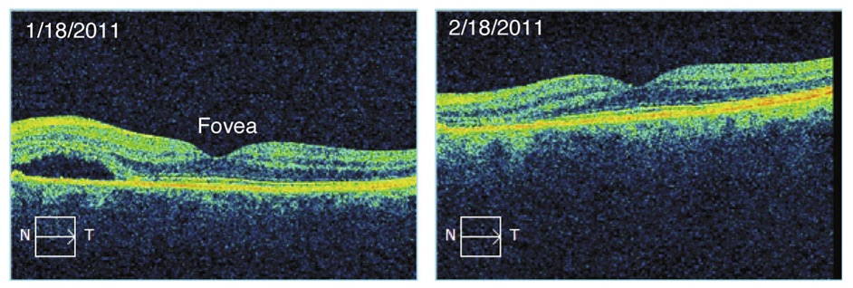
3. Figure 14.16. Color! This optical coherence tomogram of the retina was supplied by Kirk Morgan. A few figures in IPMB go beyond black and white, but this is the only one in glorious full color.

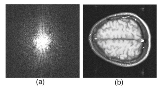
2. Figure 12.6. I like this magnetic resonance image of the brain because it helps build insight into how an image and its Fourier transform are related. It is the first of a series of six images in Chapter 12 prepared by Tuong Huu Le (University of Minnesota, also thanks to Xiaoping Hu) that, by themselves, provide a short course in image processing.

And the winner is….

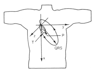
1. Figure 7.16. This picture of the direction of the dipole during the cardiac cycle nicely summarizes the electrocardiogram. My career has focused on the bioelectric behavior of the heart, so it is fitting that my top pick builds on that theme. The reason I chose it, however, is because it was on the cover of the first edition of IPMB, which I used in my first medical physics course taught by John Wikswo at Vanderbilt University.