Friday, November 24, 2023

The Deadly Rise of Anti-Science

The Deadly Rise of Anti-Science, by Peter Hotez, superimposed on Intermediate Physics for Medicine and Biology.
The Deadly Rise of Anti-Science,
by Peter Hotez.
This week I read The Deadly Rise of Anti-Science: A Scientist’s Warning, by Peter Hotez. Every American should read this book. In his introductory chapter, Hotez writes
This is a dark and tragic story of how a significant segment of the population of the United States suddenly, defiantly, and without precedent turned against biomedical science and scientists. I detail how anti-science became a dominant force in the United States, resulting in the deaths of thousands of Americans in 2021 and into 2022, and why this situation presents a national emergency. I explain why anti-science aggression will not end with the COVID-19 pandemic. I believe we must counteract it now, before something irreparable happens to set the country on a course of inexorable decline…

The consequences are shocking: as I will detail, more than 200,000 Americans needlessly lost their lives because they refused a COVID-19 vaccine and succumbed to the virus. Their lives could have been saved had they accepted the overwhelming scientific evidence for the effectiveness and safety of COVID-19 immunization or the warnings from the community of biomedical scientists and public health experts about the dangers of remaining unvaccinated. Ultimately, this such public defiance of science became a leading killer of middle-aged and older Americans, more than gun violence, terrorism, nuclear proliferation, cyberattacks or other major societal threats.
Where did this 200,000 number come from? On page 2 of Intermediate Physics for Medicine and Biology, Russ Hobbie and I claim that
One valuable skill in physics is the ability to make order-of-magnitude estimates, meaning to calculate something approximately right.

Hotez gives a classic example of estimation when deriving the 200,000 number. First, he notes that 245,000 Americans died of covid between May 1 and December 31, 2021. Covid arrived in the United States in early 2020, but vaccines did not become widely available until mid 2021. Actually, the vaccines were ready in early 2021 (I had my first dose on March 20), but May 1 was the date when the vaccine was available to everyone. During the second half of 2021, about 80% of Americans who died of covid were unvaccinated. So, Hotez multiplies 245,000 by 0.8 to get 196,000 unvaccinated deaths. After rounding this off to one significant figure, this is where he gets the number 200,000.

There are a few caveats. On the one hand, our estimate may be too high. The vaccine is not perfect. If all of the 200,000 unvaccinated people who died would have gotten the vaccine, some of them would still have perished from covid. If we take the vaccine as being 90% effective against death, we would multiple 196,000 times 0.9 to get 176,400. On the other hand, our estimate may be too low. Covid did not end on January 1, 2022. In fact, the omicron variant swept the country that winter and at its peak over 2000 people died of covid each day. So, the total covid deaths since the vaccine became available—the starting point of our calculation—is certainly higher than 245,000.

As Hotez points out, other researchers have also estimated the number of unnecessary covid deaths, using slightly different assumptions, and all the results are roughly consistent, around 200,000. (Hotez’s book appears to have been written in mid-to-late 2022; I suspect the long tail of covid deaths since then would not make much difference to this estimation, but I’m not sure.) 

In the spirit of an order-of-magnitude estimate, one should not place too great an emphasis on the precise number. It was certainly more than twenty thousand and it was without a doubt less than two million. I doubt we’ll ever know if the “true” amount is 187,000 or 224,000 or any other specific value. But we can say with confidence that about a couple hundred thousand Americans died unnecessarily because people were not vaccinated. Hotez concludes

That 200,000 unvaccinated Americans gave up their lives needlessly through shunning COVID-19 vaccines can and should haunt our nation for a long time to come.

Infectious disease scientists such as Peter Hotez, Tony Fauci, and others are true American heroes. That far-right politicians and journalists vilify these researchers is despicable and disgusting. We all owe these scientists so much. Last Monday was “Public Health Thank You Day” and yesterday was Thanksgiving. I can think of no one more deserving of our thanks than the scientists who led the effort to vaccinate America against covid. 

Why Science Isn’t Up for Debate, with Peter Hotez.

https://www.youtube.com/watch?v=PbGfeksduGE

Friday, November 17, 2023

Gustav Bucky and the Antiscatter Grid

An antiscatter grid, as discussed in Intermediate Physics for Medicine and Biology.
An antiscatter grid.
Episcophagus, CC BY-SA 4.0,
via Wikimedia Commons
.
In Chapter 16 of Intermediate Physics for Medicine and Biology, Russ Hobbie and I discuss the antiscatter grid used in radiography.

Since the radiograph assumes that photons either travel in a straight line from the point source in the x-ray tube to the detector or are absorbed, Compton-scattered photons that strike the detector reduce the contrast and contribute an overall background darkening. This effect can be reduced by placing an antiscatter grid (or radiographic grid, or “bucky” after its inventor, Gustav Bucky) just in front of the detector.
Who is Gustav Bucky? We can learn more about his life and work by examining the chapter “Two Centenaries: William Coolidge & Gustav Bucky,” by Elizabeth Beckmann and Adrian Thomas, in The Story of Radiology (Volume 2), published by the European Society of Radiology. Beckmann and Thomas begin
Gustav Peter Bucky was born on September 3, 1880 in Leipzig, Germany. He wanted to be an engineer, however at the insistence of his parents he transferred to study medicine at the University of Leipzig, graduating in1906. The combination of his interest in photography at school, his ambition to be an engineer and his parent’s insistence that he study medicine would lead him into the relatively new technical branch of medicine which was to be called radiology.
I’ve seen many reasons for scientists to straddle between physics/engineering and biology/medicine. In Bucky’s case the reason was parental pressure.

Beckmann and Thomas of course mention Bucky’s biggest contribution to science, his antiscatter grid.
It was Gustav Bucky who realised that the main problem was finding a way to reduce the scattered radiation that was responsible for the loss of definition of the radiological image from reaching the film. However, this had to be achieved with minimum impact on the primary x-ray beam. Bucky had his original idea on how to achieve this in 1909, but it took some years of experimenting for him to develop his design.

Bucky described his original design for the ‘Bucky Diaphragm’ as a ‘honeycomb’ lead grid, but with individual elements being square in shape, rather than hexagonal. He used lead since it was a material which absorbed x-rays. In this design the lead strips were thick and spaced 2 cm apart, running both parallel to the length and width of the film. This resulted in the lines of the grid being visible on the x-ray film. Despite this, the grid was effective and did remove scatter and improve image contrast.
You can eliminate those artifact lines by moving the grid.
In 1920, the American Hollis Potter further developed the grid. Potter aligned the lead strips so that they now ran in one direction only, and he also made the lead strips thinner so that they were less visible on the image. Potter also proposed moving the grid during exposure, which blurred out the image of the lead strips on the radiographic image... The resulting moving grid, based upon the work of Bucky and Potter, became known as the Potter-Bucky grid.
Albert Einstein and Gustav Bucky,
Leo Baeck Institute, F 5347B.
Bucky moved from Germany to the United States in 1929. He became good friends with Albert Einstein.
In 1933, Bucky met up again with his friend Albert Einstein when he arrived in New York. When on holiday together Gustav and Albert would go for a long walk together each day, discussing and developing new ideas…

Probably the most famous collaboration between Bucky and Einstein was the idea of ‘a light intensity self-adjusting camera’ with a US patent granted on October 27, 1936...

It is a sign of the close relationship between Bucky and Einstein that Bucky visited Einstein every day during his final illness and was at the hospital only hours before Einstein’s death in April 1955.
The story concludes
Gustav Bucky was a friendly, modest, undemanding person who made a lasting and significant contribution to radiology. For 21st century radiology the impact of the invention for which Gustav Bucky is most remembered – the Bucky Grid – continues. The grid is as important in modern digital detection systems, like computed radiography (CR) plates or digital radiography (DR) detector systems, as it was with x-ray film in the 1920s. 

Friday, November 10, 2023

Monet's Water Lilies

When my wife and I were in Paris several years ago we visited the Musée de l’Orangerie, where Claude Monet’s beautiful water lily murals are displayed. Monet (1840–1926) is the famous impressionist painter who, during the last decades of his life, painted lilies floating on the surface of the pond at his home in Giverny. I remember sitting in one of the oval rooms staring at these giant paintings. It was so quiet and peaceful.

Monet’s water lily murals in the Musée de l’Orangerie in Paris
Monet’s water lily murals in the Musée de l’Orangerie in Paris.
Brady Brenot, CC BY-SA 4.0 , via Wikimedia Commons.

Water lilies take advantage of some interesting physics. First, their stalks and leaves contain air pockets, reducing their average density and making them buoyant. Russ Hobbie and I compare the effect of buoyancy in terrestrial and aquatic animals. I quote this comparison below, but I have replaced the word “animals” by “plants”.

Plants are made up primarily of water, so their density is approximately 103 kg m−3. The buoyant force depends on the plant’s environment. Terrestrial plants live in air, which has a density of 1.2 kg m−3. The buoyant force on terrestrial plants is very small compared to their weight. Aquatic plants live in water, and their density is almost the same as the surrounding fluid. The buoyant force almost cancels the weight, so the plant is essentially “weightless.” Gravity plays a major role in the life of terrestrial plants, but only a minor role for aquatic plants. Denny (1993) explores the differences between terrestrial and aquatic plants in more detail.

Another piece of physics important to water lilies is surface tension, a topic only briefly mentioned in the fifth edition of Intermediate Physics for Medicine and Biology, but which (spoiler alert!) may play a larger role in the sixth edition. The lily’s leaf is waxy, which repels water and enhances its ability to remain on the water-air surface. In addition, small cilia increase the surface area.

A last bit of physics has to do with the surface-to-volume ratio. Usually surface tension can’t support a large object, because its weight increases with the cube of its linear size, whereas the effect of surface tension increases with the object’s perimeter. Therefore, the impact of gravity increases with size more dramatically than does the impact of surface tension, so a large object sinks like a rock. The water lily’s leaf, however, is thin, and making the leaf larger increases its surface area but not its thickness. The weight only increases as the square of its linear size, not as the cube. If the leaf is large enough, gravity will still win out, but the leaf can be larger than you might expect and still float on the water surface.

Monet donated his water lily murals to France at the end of World War I, to create a place where people could reflect on those who gave their life for the nation. When visiting them, you can also contemplate the role of physics in medicine and biology.

Happy Veterans Day.

One of Monet’s water lily murals at the Musée de l’Orangerie.

Monet’s Water Lilies: Great Art Explained.

Friday, November 3, 2023

The Golay Coil

Last week I introduced the Helmholtz coil and the Maxwell coil. The Maxwell coil is useful for creating the magnetic field gradient needed for magnetic resonance imaging. At the end of the post, I wrote
The Maxwell coil is great for producing the magnetic field gradient dBz/dz needed for slice selection in MRI, but what coil is required to produce the gradients dBz/dx and dBz/dy needed during MRI readout and phase encoding? That, my friends, is a story for another post.
Today, I will finish the story.

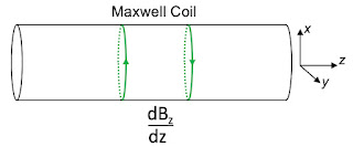
First, let’s assume the gradient coils are all located on the surface of a cylinder. If this were a clinical MRI scanner, the person would lie on a bed that would be slid into the cylinder to get an image. The Maxwell coil consists of two circular coils, separated by a distance equal to the square root of three times the coil radius. The parts of the coil in the back that are hidden by the cylinder are shown as dashed. The two coils carry current in opposite directions, as shown below, creating a gradient dBz/dz in the imaging region midway between the two coils on the axis of the cylinder.

A Maxwell coil.

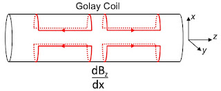
To perform imaging, however, you need gradients in the x and y directions too. To create dBz/dx, you typically use what is called a Golay coil. It consists of four coils wound on the cylinder surface as shown below. 

A Golay coil.

The mathematics to determine the details of this design is too complicated for this post. Suffice to so, it requires setting the third derivative of Bz with respect to x equal to zero. The resulting coils should each subtend an angle of 120°. Their inner loops should be separated by 0.778 cylinder radii, and their outer loops by 5.14 radii.

To create the gradient dBz/dy, simply rotate the Golay coil by 90°, as shown below. 

A rotated Golay coil.

So, to perform magnetic resonance imaging you need a nested set of three coils as shown below. 

A set of three gradient coils used in MRI.

The picture gets confusing with all the hidden lines. Here is how the set looks with the hidden parts of the coils truly hidden.

A set of three gradient coils used in MRI (hidden lines removed).

While this set of coils will produce linear magnetic field gradients in the central region, in state-of-the-art MRI scanners the coils are somewhat more complicated, with multiple loops corresponding to each loop shown above.

We all know who Helmholtz and Maxwell are, but who is Golay? Marcel J. E. Golay (1902-1989) was a Swiss scientist who came to the US to get his PhD at the University of Chicago and then stayed. He had a varied career, making fundamental advances in chromatography, information theory, and the detection of infrared light. He studied the process of shimming: making small adjustments to the magnetic field of a MRI scanner to make the static field more homogeneous. This work ultimately led to the design of gradient coils.

In Chapter 18 of Intermediate Physics for Medicine and Biology, Russ Hobbie and I discuss magnetic resonance imaging and the need for magnetic field gradients. In a nutshell, MRI converts magnetic field strength to spin precession frequency. By measuring this frequency, you can obtain information about magnetic field strength. A magnetic field gradient lets you map frequency to position, an idea which is at the heart of imaging using magnetic resonance.

Friday, October 27, 2023

The Helmholtz Coil and the Maxwell Coil

To do magnetic resonance imaging, you need a static magnetic field that is uniform and a switchable magnetic field that has a uniform gradient. How do you produce such fields? In this post, I explain one of the simplest ways: using a Helmholtz coil and a Maxwell coil.

Both of these are created using circular coils. The magnetic field Bz produced by a circular coil can be calculated using the law of Biot and Savart (see Chapter 8 of Intermediate Physics for Medicine and Biology)

where μ0 is the permeability of free space (the basic constant of magnetostatics), I is the coil current, N is the number of turns, R is the coil radius, and z is the distance along the axis from the coil center.

The Helmholtz Coil

The Helmholtz coil consists of two circular coils in parallel planes, having the same axis and the same current in the same direction, that are separated by a distance d. Our goal will be to find the value of d that gives the most uniform magnetic field. By superposition, the magnetic field is 


To create a uniform magnetic field, we will perform a Taylor expansion of the magnetic field about the origin (z = 0). We will need derivatives of the magnetic field. The first derivative is


(The reader will have to fill in the missing steps when calculating these derivatives.) At z = 0, this derivative will go to zero. In fact, because the magnetic field is even about the z axis, all odd derivatives will be zero, regardless of the value of d.

The second derivative is

At z = 0, the two terms in the brackets are the same. Our goal is to have this term be zero, implying that the second order term in the Taylor series vanishes. This will happen if

or, in other words, d = R. This famous result says that for a Helmholtz pair the coil separation should equal the coil radius.

A Helmholtz coil produces a remarkably uniform field near the origin. However, it is not uniform enough for use in most magnetic resonance imaging machines, which typically have a more complex set of coils to create an even more homogeneous field. If you need a larger region that is homogeneous, you could always just use a larger Helmholtz coil, but then you would need more current to achieve the desired magnetic field at the center. A Helmholtz pair isn’t bad if you want to use only two reasonably sized coils.

The Maxwell Coil

The Helmholtz coil produces a uniform magnetic field, whereas the Maxwell coil produces a uniform magnetic field gradient. It consists of two circular coils, in parallel planes having the same axis, that are separated by a distance d, but which have current in the opposite directions. Again, our goal will be to find the value of d that gives the most uniform magnetic field gradient. The magnetic field is


The only difference between this case and that for the Helmholtz coil is the change in sign of the second term in the bracket. If z = 0, the magnetic field is zero. Moreover, the magnetic field is an odd function of z, so all even derivatives also vanish. The first derivative is


This expression gives us the magnitude of the gradient at the origin, but it doesn’t help us create a more uniform gradient. The second derivative is


This derivative is zero at the origin, regardless of the value of d. So, we have to look at the third derivative.


At z = 0, this will vanish if
or, in other words, d = √3 R = 1.73 R. Thus, the two coils have a greater separation for a Maxwell coil than for a Helmholtz coil. The Maxwell coil would be useful for producing the slice selection gradient during MRI (for more about the need for gradient fields in MRI, see Chapter 18 of IPMB).

Conclusion

Below is a plot of the normalized magnetic field as a function of z for the Helmholtz coil (blue) and the Maxwell coil (yellow). As you can see, the region with a uniform field or gradient is small. It depends on what level of accuracy you need, but if you are more than half a radius from the origin you will see significant deviations from homogeneity.
 

Russ Hobbie and I never discuss the Helmholtz coil in Intermediate Physics for Medicine and Biology. We don’t mention the Maxwell coil by name, but Problem 33 of Chapter 18 analyzed a Maxwell pair even if we don’t call it that.

The Maxwell coil is great for producing the magnetic field gradient dBz/dz needed for slice selection in MRI, but how do you produce the gradients dBz/dx and dBz/dy needed during MRI readout and phase encoding? That, my friends, is a story for another post.

Friday, October 20, 2023

Mr. Clough

A teacher affects eternity; he can never tell where his influence stops. 

Henry Adams

Stephen Clough, from the 1975
Homestead Jr.-Sr. High School Yearbook.
How does someone end up being coauthor on a textbook like Intermediate Physics for Medicine and Biology? It takes a lot of friends, teachers, and role models who help you along the way. I had many excellent teachers when I was young. One of the best was Stephen Clough.

I attended grades 7–10 at Homestead Junior-Senior High School. Usually a junior high and senior high are in separate buildings, but the suburb of Fort Wayne where I lived at the time was new and growing, and had the two combined. For two years (I think grades 9 and 10) I had English with Mr. Clough. He was one of the younger teachers and had longish hair and a mustache, and I thought he was little bit of a hippie. That’s OK, because in the mid 70s hippies were still groovy (although they would go out of fashion soon).

Before I had Mr. Clough, I didn’t read much. I was obsessed with baseball and would read an occasional sports biography, but not much else. I did well in school, but I don’t remember our classes being too challenging or having much homework. Life was about hanging around with friends, playing ping pong, riding bikes, listening to music, and watching television. But Mr. Clough had us reading modern fiction, like Animal Farm and Lord of the Flies. For me, this was an intellectual awakening. Before Mr. Clough I rarely read books; after Mr. Clough I read all the time (and still do).
Me (age 15) from the 1975
Homestead Jr.-Sr. High School Yearbook.

I remember how, on Fridays, Mr. Clough would bring his guitar to school and play for us and sing. I thought this was the coolest thing I’d ever seen. None of my other teachers related to us like that. He played a lot of Dylan. I’ll never forget the day he explained what the words meant in the song American Pie

Mr. Clough had a huge influence on my academic development. Reading books led to reading the scientific writing of Isaac Asimov, which led to majoring in physics in college, which led to a PhD, which ultimately led to becoming a coauthor of Intermediate Physics for Medicine and Biology. I owe him much.

As Henry Adams said, a teacher affects eternity. I hope everyone teaching a class using IPMB keeps that in mind. You can never tell where your influence stops. 

I last saw Mr. Clough at my 30th high school reunion. My friend from high school, Dave Small, became an opera singer, and he sang several songs for us at the gathering. Guess who accompanied him on the guitar? Stephen Clough.

American Pie, by Don McLean.

https://www.youtube.com/watch?v=PRpiBpDy7MQ

Friday, October 13, 2023

J. Robert Oppenheimer, Biological Physicist

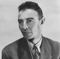
J. Robert Oppenheimer.
Did you watch Oppenheimer in the theater this summer? I did. The movie told how J. Robert Oppenheimer led the Manhattan Project that built the first atomic bomb during World War II. But the movie skipped Oppenheimer’s research in biological physics related to photosynthesis.

Russ Hobbie and I only make a passing mention of photosynthesis in Chapter 3 of Intermediate Physics for Medicine and Biology.
The creation of glucose or other sugars is the reverse of the respiration process and is called photosynthesis. The free energy required to run the reaction the other direction is supplied by light energy.
From Photon to Neuron: Light, Imaging, Vision, by Philip Nelson, superimposed on Intermediate Physics for Medicine and Biology.
From Photon to Neuron,
by Philip Nelson.
To learn more about Oppie and photosynthesis, I turn to Philip Nelson’s wonderful textbook From Photon to Neuron: Light, Imaging, Vision. His discussion of photosynthesis begins
Photosynthetic organisms convert around 1014 kg of carbon from carbon dioxide into biomass each year. In addition to generating the food that we enjoy eating, photosynthetic organisms emit a waste product, free oxygen, that we enjoy breathing. They also stabilize Earth’s climate by removing atmospheric CO2.
Nelson begins the story by introducing William Arnold, Oppenheimer’s future collaborator.
W. Arnold was an undergraduate student interested in a career in astronomy. In 1930, he was finding it difficult to schedule all the required courses he needed for graduation. His advisor proposed that, in place of Elementary Biology, he could substitute a course on Plant Physiology organized by [Robert] Emerson. Arnold enjoyed the class, though he still preferred astronomy. But unable to find a place to continue his studies in that field after graduation, he accepted an offer from Emerson to stay on as his assistant.
Emerson and Arnold went on to perform critical experiments on photosynthesis. Then Emerson performed another experiment with [Charlton] Lewis, in which they found that chlorophyll does not absorb light with a wavelength of 480 nm (blue), but an accessory pigment called phycocyanin does. Emerson and Lewis concluded that “the energy absorbed by phycocyanin must be available for photosynthesis.”

Here is where Oppenheimer comes into the story. I will let Nelson tell it.
Could phycocyanin absorb light energy and somehow transfer it to the chlorophyll system?...

Arnold eventually left Emerson’s lab to study elsewhere, but they stayed in contact. Emerson told him about the results with Lewis, and suggested that he think about the energy-transfer problem. Arnold had once audited a course on quantum physics, so he visited the professor for that course to pose the puzzle. The professor was J. R. Oppenheimer, and he did have an idea. Oppenheimer realized that a similar energy transfer process was known in nuclear physics; from this he created a complete theory of fluorescence resonance energy transfer. Oppenheimer and Arnold also made quantitative estimates indicating that phycocyanin and chlorophyll could play the roles of donor and acceptor, and that this mechanism could give the high transfer efficiency needed to explain the data.
So, what nuclear energy transfer process was Oppenheimer talking about? In Arnold and Oppenheimer’s paper, they wrote
It is the purpose of the present paper to point out a mechanism of energy transfer from phycocyanin to chlorophyll, the efficiency of which seems to be high enough to account for the results of Emerson and Lewis. This new process is, except for the scale, identical with the process of internal conversion that we have in the study of radioactivity.
Internal conversion is a topic Russ and I address in IPMB. We said
Whenever a nucleus loses energy by γ decay, there is a competing process called internal conversion. The energy to be lost in the transition, Eγ, is transferred directly to a bound electron, which is then ejected.
Introductory Nuclear Physics by Kenneth Krane, superimposed on Intermediate Physics for Medicine and Biology.
Introductory Nuclear Physics,
by Kenneth Krane.
More detail can be found in Introductory Nuclear Physics by Kenneth Krane.
Internal conversion is an electromagnetic process that competes with γ emission. In this case the electromagnetic multipole fields of the nucleus do not result in the emission of a photon; instead, the fields interact with the atomic electrons and cause one of the electrons to be emitted from the atom. In contrast to β decay, the electron is not created in the decay process but rather is a previously existing electron in an atomic orbit. For this reason internal conversion decay rates can be altered slightly by changing the chemical environment of the atom, thus changing somewhat the atomic orbits. Keep in mind, however, that this is not a two-step process in which a photon is first emitted by the nucleus and then knocks loose an orbiting electron by a process analogous to the photoelectric effect; such a process would have a negligibly small probability to occur.
Nelson compares the photosynthesis process to another process widely used in biological imaging: Fluorescence resonance energy transfer (FRET). He describes FRET this way.
We can find pairs of molecular species, called donor/acceptor pairs, with the property that physical proximity abolishes fluorescence from the donor. When such a pair are close, the acceptor nearly always pulls the excitation energy off the donor, before the donor has a chance to fluoresce. The acceptor may either emit a photon, or lose its excitation without fluorescence (“nonradiative” energy loss).
Let’s put this all together. The donor in FRET is like the phycocyanin molecule in photosynthesis is like the nucleus in internal conversion. The acceptor in FRET is like the chlorophyll molecule in photosynthesis is like the electron cloud in internal conversion. The fluorescence of the donor/phycocyanin/nucleus is suppressed (in the nuclear case, fluorescence would be gamma decay). Instead, the electromagnetic field of the donor/phycocyanin/nucleus interacts with, and transfers energy to, the acceptor/chlorophyll/electron cloud. In the case of FRET, the acceptor then fluoresces (which is what is detected when doing FRET imaging). The chlorophyll/electron cloud does not fluoresce, but instead ejects an electron in the case of internal conversion, or energizes an electron that can ultimately perform chemical reactions in the case of photosynthesis. All three processes are exquisitely sensitive to physical proximity. For FRET imaging, this sensitivity allows one to say if two molecules are close to each other. In photosynthesis, it means the chlorophyll and phycocyanin must be near one another. In internal conversion, it means the electrode cloud must overlap the nucleus, which implies that the process usually results in emission of a K-shell electron since those innermost electrons have the highest probability of being near the nucleus.

There’s lots of interesting stuff here: How working at the border between disciplines can result in breakthroughs; how physics concepts can contribute to biology; how addressing oddball questions arising from data can lead to new breakthroughs; how quantum mechanics can influence biological processes (Newton rules biology, except when he doesn’t); how seemingly different phenomena—such as FRET imaging, photosynthesis, and nuclear internal conversion—can have underlying similarities. I wish my command of quantum mechanics was strong enough that I could explain all these resonance effects to you in more detail, but alas it is not.

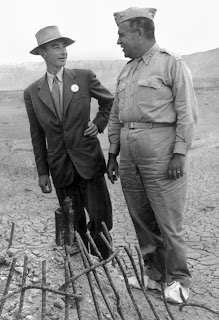
Oppenheimer and General Groves at the Trinity test site.
Oppenheimer and General Groves
at the Trinity test site. I love
Oppie’s pork pie hat.
If you haven’t seen Oppenheimer yet, I recommend you do. Go see Barbie too. Make it a full Barbenheimer. But if you want to learn about the father of the atomic bomb’s contributions to biology, you’d better stick with From Photon to Neuron or this blog. 


The official trailer to Oppenheimer.

https://www.youtube.com/watch?v=bK6ldnjE3Y0


Photosynthesis.

https://www.youtube.com/watch?v=jlO8NiPbgrk&t=14s

Friday, October 6, 2023

The Dobson Unit

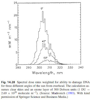
Figure 14.28 from Intermediate Physics for Medicine and Biology, showing the spectral dose rate weighted for ability to damage DNA.
In Chapter 14 of Intermediate Physics for Medicine and Biology, Russ Hobbie and I discuss the risk of DNA damage—and therefore cancer—caused by ultraviolet light from the sun. Figure 14.28 in IPMB presents the results of a calculation of UV dose rate, weighted for DNA damage. The caption of the figure states “the calculation assumes clear skies and an ozone layer of 300 Dobson units (1 DU = 2.69 × 10²⁰ molecule m-2).”

The Dobson Unit, what’s that?

Rather than explaining it myself, let me quote the NASA website about ozone.
What is a Dobson Unit?

The Dobson Unit is the most common unit for measuring ozone concentration. One Dobson Unit is the number of molecules of ozone [O3] that would be required to create a layer of pure ozone 0.01 millimeters thick at a temperature of 0 degrees Celsius and a pressure of 1 atmosphere (the air pressure at the surface of the Earth). Expressed another way, a column of air with an ozone concentration of 1 Dobson Unit would contain about 2.69 × 10¹⁶ ozone molecules for every square centimeter of area at the base of the column. Over the Earth’s surface, the ozone layer’s average thickness is about 300 Dobson Units or a layer that is 3 millimeters thick.

The Dobson Unit was named after British physicist and meteorologist Gordon Miller Bourne Dobson (1889 –1976) who did early research on ozone in the atmosphere.

Worried about climate change? The ozone story may provide some hope. When man-made chemicals such as chlorofluorocarbons, for example freon, are released into the atmosphere, they damage the ozone layer, allowing larger amounts of ultraviolet radiation to reach the earth’s surface. In the 1970s, an ozone hole developed each year over the south pole. In 1987, countries from all over the world united to pass the Montreal Protocol, which banned many ozone depleting substances. Since that time, the ozone hole has been getting smaller. This represents a success story demonstrating how international cooperation can address critical environmental hazards. Now, we need to do the same thing for greenhouse gases to combat climate change. 


How the ozone layer was discovered.

https://www.youtube.com/watch?v=GS0dilngPws


Don't let this happen to your planet!

https://www.youtube.com/watch?v=nCpH71npnvo

Friday, September 29, 2023

Decay Plus Input at a Constant Rate Revisited

In Chapter 2 of Intermediate Physics for Medicine and Biology, Russ Hobbie and I discuss the problem of decay plus input at a constant rate.
Suppose that in addition to the removal of y from the system at a rate –by, y enters the system at a constant rate a, independent of y and t. The net rate of change of y is given by

Then we go on to discuss how you can learn things about a differential equation without actually solving it.

It is often easier to write down a differential equation describing a problem than it is to solve it… However, a good deal can be learned about the solution by examining the equation itself. Suppose that y(0) = 0. Then the equation at t = 0 is dy/dt = a, and y initially grows at a constant rate a. As y builds up, the rate of growth decreases from this value because of the –by term. Finally when a by = 0, dy/dt is zero and y stops growing. This is enough information to make the sketch in Fig. 2.13.

The equation is solved in Appendix F. The solution is
… The solution does have the properties sketched in Fig. 2.13, as you can see from Fig. 2.14.
Figure 2.13 looks similar to this figure
Sketch of the initial slope a and final value a/b of y when y(0) = 0. In this figure, a=b=1.

 And Fig. 2.14 looks like this

A plot of y(t) using Eq. 2.26, with a=b=1.

However, Eq. 2.26 is not the only solution that is consistent with the sketch in Fig. 2.13. Today I want to present another function that is consistent with Fig. 2.13, but does not obey the differential equation in Eq. 2.25.

Let’s examine how this function behaves. When bt is much less than one, the function becomes y = at, so it’s initial growth rate is a. When bt is much greater than one, the function approaches a/b. The sketch in Fig. 2.13 is consistent with this behavior.

Below I show both Eqs. 2.26 and 2.26’ in the same plot.

A plot of y(t) using Eq. 2.26 (blue) and Eq. 2.26' (yellow), with a=b=1.

The function in Eq. 2.26 (blue) approaches its asymptotic value at large t more quickly than the function in Eq. 2.26’ (yellow).

The moral of the story is that you can learn a lot about the behavior of a solution by just inspecting the differential equation, but you can’t learn everything (or, at least, I can’t). To learn everything, you need to solve the differential equation. 

By the way, if Eq. 2.26’ doesn’t solve the differential equation in Eq. 2.25, then what differential equation does it solve? The answer is

 How did I figure that out? Trial and error.

Friday, September 22, 2023

The Slide Rule

In Chapter 2 of Intermediate Physics for Medicine and Biology, Russ Hobbie and I discuss semilog plots, where the vertical axis is marked using a logarithmic scale. In this case, a constant distance along the vertical axis corresponds to a constant multiple in the numerical value. In other words, the distance between 1 and 2 is the same as the distance between 2 and 4, which is the same as the distance between 4 and 8, and so on. Looking at a semilog plot helps the reader get a better understanding of how logarithms and exponentials work. Yet, what would be a really useful learning tool is not something readers just look at, but something that they can hold in their hands, something they can manipulate, something they can touch.

Enter the slide rule. Sixty years ago, when electronic calculators did not yet exist, the slide rule is how scientists and engineers performed calculations. I didn’t use a slide rule in school. I’m from the first generation that had access to electronic calculators. They were expensive but not prohibitively so, and we all used them. But my dad used a slide rule. He gave me his, mainly as an artifact of a bygone era. I rarely use it but I have kept it in honor of him. It was made by the Keuffel & Esser Company in New York. It is a fairly fancy one and has a variety of different scales.

First, let’s look at the C and D scales. These are marked logarithmically, just like semilog paper. In fact, if you wanted to draw you own semilog graph paper, you could take out my dad’s slide rule, hold it vertical, and mark off the tick marks on your plot axis. On dad’s slide rule, C and D are both marked logarithmically, but they can move relative to each other. Suppose you wanted to prove that the distance between 1 and 2 is the same as the distance between 2 and 4. You could slide the C scale so that its 1 lined up with the 2 on the fixed D scale. If you do this, then the 2 on the C scale really does line up with the 4 on the D scale, and the 4 on the C scale matches the 8 on the D scale. The value on the D scale is always twice the value on the C scale. When you think about it, you have just invented a way to multiply any number by 2. 

A slide rule, showing how to multiply by 2.
A slide rule showing how to multiply by 2.

This trick of doing multiplication isn’t just for multiplying by 2. Suppose you wanted to multiply 1.7 by 3.3. You could line the 1 on the C scale up with 1.7 on the D scale, and then look at what value on the D scale corresponds to 3.3 on the C scale. The slide rule has a handy little ruled glass window called the cursor that you can use to read the D scale accurately (if the cursor lands between two tick marks, don’t be afraid to estimate an extra significant figure based on where it is between ticks). I get 5.60. Use you calculator and you get 5.61. The slide rule is not exact (my answer was off by 0.2%) but you can get an excellent approximation using it. If my eyes weren’t so old, or if I had a more powerful set of reading glasses, I might have gotten a answer that was even closer. I bet with practice you young folks with good eyes and steady hands could routinely get 0.1% accuracy.

A slide rule showing how to multiply 1.7 by 3.3.

If you can do multiplication, then you can do its inverse: division. To calculate 8.2/4.5, move the cursor to 8.2 on the D scale, then slide the C scale until 4.5 aligns with the cursor. Then read the value on the D scale that aligns with 1 on the C scale. I get 1.828. My calculator says 1.822. When using the slide rule, you need to estimate your result to get the decimal place correct. How do you know the answer is 1.828 and not 18.28 or 0.1828? Well, the answer should be nearly 8/4 = 2, so 1.828 must be correct. Some would claim that the extra step of requiring such an order-of-magnitude estimate is a disadvantage of the slide rule. I say that even when using an electronic calculator you should make such estimates. It’s too easy to slip a decimal point somewhere in the calculation, and you always want to have a rough idea of what result you expect to avoid embarrassing mistakes. Think before you calculate! 

A slide rule showing how to divide 8.2 by 4.5.

Suppose you have a number like 5.87 and you want to know its reciprocal. You could, of course, just calculate 1/5.87. But like most scientific calculators that have a special reciprocal key, dad’s slide rule has a special CI scale that performs the calculation quickly. The CI scale is merely the mirror image of the C scale; it is designed logarithmically, but from right to left rather than from left to right. Put the cursor at 5.87 on the CI scale, and then read the value of the C scale (no sliding required). I read 1.698. I estimate that 1/5 is about 0.2, so the result must really be 0.1698. My electronic calculator says 0.1704.

A slide rule showing how to calculate the reciprocal of 5.89.

One property of logarithms is that log(x2) = 2 log(x). To calculate squares quickly use the A scale (on my dad’s slide rule the A scale is on the flip side), which is like the C or D scales except that two decades are ruled over A whereas just one is over D. If you want 15.92, put 1.59 on the D scale and read 2.53 on the A scale (again, no sliding). You know that 162 is 256, so the answer is 253. My calculator says 252.81. Not bad.

A slide rule showing how to calculate the square of 15.9.

If you can do squares, you can do square roots. To calculate the square root of 3261, place the cursor at 3.261 on the A scale. There is some ambiguity here because the A scale has two decades so you don’t know which decade to use. For reasons I don’t really understand yet, use the rightmost decade in this case. Then use the cursor to read off 5.72 on the C scale. You know that the square root of 3600 is 60, so the answer is 57.2. My calculator says 57.105. 

A slide rule showing how to calculate the square root of 3261.

There are additional scales to calculate other quantities. The L scale is ruled linearly and can be used with the C scale to compute logarithms to base 10. Other scales can be used for trig functions or powers.

A TI-30 electronic calculator, superimposed on the cover of Intermediate Physics for Medicine and Biology.
I don’t recommend giving up your TI-30 for a slide rule. However, you might benefit by spending an idle hour playing around with an old slide rule, getting an intuitive feeling for logarithmic scaling. You’ll never look at a semilog plot in the same way again.


How to use a slide rule.

https://www.youtube.com/watch?v=xYhOoYf_XT0