More About Implantable Microcoils for Intracortical Magnetic Stimulation

Three years ago, I wrote a post in this blog discussing an article by Seung Woo Lee and his coworkers (“Implantable Microcoils for Intracortical Magnetic Stimulation,” Science Advances, 2:e1600889, 2016). They claimed to have performed magnetic stimulation of nerves by passing a 40 mA, 3 kHz current through a single-turn microcoil with a size less than a millimeter. I claimed that the electric field induced in the surrounding tissue by such a coil would be much smaller than Lee et al. predicted. In their Figure 2 they calculated that a 1 mA current induced an electric field on the order of 2 V/m. I calculated an electric field about a million times smaller, and concluded “their results are too strange to believe and too important to ignore.”

I didn’t ignore them. Recently a graduate student here at Oakland University, Mohammed Alzahrani, and I tested the hypothesis that excitation using microcoils is caused by capacitive coupling rather than magnetic stimulation. The picture below shows our model. The current at the left end of the microcoil passes through the capacitance of the insulation and enters the surrounding tissue. It then flows through the tissue, possibly exciting neurons along its path, until reentering the wire through the capacitance near the right end.

Does this model look familiar? It’s similar to the cable model for a nerve axon (for more about the cable model, see Section 6.11 of Intermediate Physics for Medicine and Biology). The wire in our model is analogous to the intracellular space of the axon in the traditional cable model, and the insulation surrounding the wire is analogous to the cell membrane. Our model’s even simpler than the traditional cable model because the conductance of the insulation is so low that it can be taken as zero; the only way for current to leave the wire is through the capacitance. This model is not new; it was derived in the 19^th century to describe current through the transatlantic telegraph cable.

Our goal was to calculate the electric field assuming capacitive coupling, to see whether it’s larger or smaller than what you’d expect from magnetic stimulation. We concluded

In summary, we predict an electric field in the tissue due to capacitive coupling of about 4 mV/m for a current of 1 mA and 3 kHz. The electric field produced by magnetic stimulation would be thousands of times less, on the order of 0.002 mV/m. Therefore, capacitive coupling should be the dominant mechanism for stimulation with a microcoil.

We haven’t published our results yet, but you can download a preprint on my ResearchGate page (doi 10.13140/RG.2.2.19222.40006). I’m curious what you think.

What’s the moral to this story? As I wrote at the end of my previous post, experiments “need to be consistent with the fundamental physical laws outlined in Intermediate Physics for Medicine and Biology.”

Isotopes to Worry About: Cesium-137, Iodine-131, and Strontium-90

Three hazardous isotopes released by a nuclear explosion or accident are cesium-137, iodine-131, and strontium-90.

Cesium-137

Isotopes with short half lives often have disappeared within days of a nuclear accident, after they emit lots of radiation. Isotopes with long half lives may linger for millennia, but aren’t very radioactive. Isotopes with half lives of a few decades are “just right” for being an environmental hazard; their lifetimes are short enough that they release a lot of radioactivity, but are long enough that they cause decades of danger. Cesium-137 (¹³⁷Cs) has a half-life of 30 years. It is the main source of remaining radiation at the site of the Chernobyl accident.

Cesium-137 is volatile, meaning it evaporates at high temperatures, allowing it to mix with the air and spread with the wind. In addition, cesium is in the same column of the periodic table as sodium and potassium, so it forms water soluble salts that distribute throughout the body. It beta decays (0.51 MeV) to a meta-stable state of barium-137, which then decays by emission of a gamma ray (0.66 MeV).

Accidental uptake of caesium-137 can be treated with Prussian blue, which binds to it and reduces its biological half-life from 70 to 30 days.

Iodine-131

Iodine-131 (¹³¹I) has a half-life of eight days, so it is dangerous for only a few weeks after a nuclear explosion or accident. However, radioactive iodine is concentrated in the thyroid gland, causing thyroid cancer. Iodine-131 undergoes beta decay (0.61 MeV) to xenon-131, which then emits a 0.36 MeV gamma ray. It’s so potent a radioisotope that it’s used for cancer therapy (see Section 17.11 of Intermediate Physics for Medicine and Biology).

After a nuclear accident, people take potassium iodide pills to flood the thyroid gland with non-radioactive iodine, suppressing the uptake of the radioactive isotope.

Strontium-90

Like cesium-137, strontium-90 (⁹⁰Sr) has a half life of about 30 years. It undergoes beta decay (0.55 MeV) to yttrium-90, which in turn beta decays (2.3 MeV) to stable zirconium-90. Strontium-90 is in the same column of the periodic table as calcium, so it is taken up by bones (it’s a “bone seeker”) and therefore has a long biological half-life (about 18 years).

Dirty Bombs

Want something to worry about? Consider this radiological nightmare: a terrorist dirty bomb consisting of equal parts cesium-137, iodine-131, and strontium-90. Good luck sleeping tonight.

Slice Selection During Magnetic Resonance Imaging

In Chapter 18 of Intermediate Physics for Medicine and Biology, Russ Hobbie and I discuss magnetic resonance imaging. The first step in most MRI pulse sequences is to excite the spins in a slice of the sample. Three magnetic fields are required: A static field B₀ in the z direction that aligns the spins, a magnetic field gradient G in the z direction that selects a slice with thickness Δz, and a radiofrequency field in the x direction B_x(t) that excites the spins.

The RF signal is called a π/2 pulse because it rotates the spins through an angle of 90 degrees (π/2 radians), from the z direction to the x-y plane. The Larmor frequency (the angular frequency at which the spins precess at the center of the slice, z = 0) is ω₀ = γB₀, where γ is the gyromagnetic ratio. Figure 18.23a of IPMB shows the RF signal as a function of time t: an oscillation at the Larmor frequency modulated by the sinc function.

Figure 18.23a of IPMB, showing the radiofrequency signal
used as a π/2 pulse during slice selection.

Figure 18.24 illustrates part of the pulse sequence, showing when the RF pulse (B_x, top) and the gradient (G, bottom) are applied.

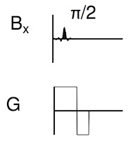From Figure 18.24 of IPMB, showing the part of the
pulse sequence responsible for slice selection.

Did you ever wonder how the spins behave during this part of the pulse sequence? Do the spins flip all at once near the center of the π/2 pulse, or gradually throughout its duration? Why is there a second negative lobe of the gradient after the π/2 pulse is complete? To answer these questions, let’s analyze slice selection using the Bloch equations—the differential equations governing how spins precess in a magnetic field. Our analysis is similar to that in Section 18.5 of IPMB. 

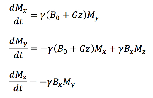
If we ignore relaxation, the Bloch equations are

where M_x, M_y, and M_z are the components of the magnetization (a measure of the average spin orientation).

Next, let’s transform to a coordinate system (M_x', M_y', M_z') rotating at the Larmor frequency. I will leave the details of the transformation to you (they are similar to those in Section 18.5.2 of IPMB). We obtain

In general the Larmor frequency γB₀ is much higher than the modulation frequency γGΔz/2 (thousands of oscillations occur within the central lobe of the sinc function rather than the dozen shown in Fig. 18.23a), so we average over many cycles (as in Section 18.5.3 of IPMB). The Bloch equations simplify to

Before we can solve this system of three coupled ordinary differential equations, we need to specify the initial conditions. At t = −∞, M_x' = M_y' = 0 and M_z' = M₀, where M₀ is the equilibrium value of the magnetization.

At this point, we define dimensionless variables

where M = (M_x, M_y, M_z). The differential equations become

where z' ranges from -1 to 1, and the initial conditions at t' = −∞ are M'_x' = M'_y' = 0 and M'_z' = 1.

I like this elegant system of equations, except all the primes are annoying. For the rest of this post I’ll drop the primes. Your job is to remember that these are dimensionless coordinates in a rotating coordinate system.

I wanted to solve these equations analytically, but couldn’t. I tried weird guesses involving the sine integral and sometimes I thought I was close, but none of my attempts worked. If you, dear reader, find an analytical solution, send it to me. You will be my hero forever.

Having no analytical solution, I wrote a simple Matlab program to solve the equations numerically.

dt=pi/1000;
T=10*pi;
nt=2*T/dt;
dz=0.05;
nz=2/dz+1;
for j=1:nz
    mx(1,j)=0;
    my(1,j)=0;
    mz(1,j)=1;
    z(j)=-1+(j-1)*dz;
    end
t(1)=-T;
for i=1:nt-1
    t(i+1)=t(i)+dt;
    for j=1:nz
        mx(i+1,j)=mx(i,j) + dt*z(j)*my(i,j);
        my(i+1,j)=my(i,j) + dt*(0.5*sin(t(i))/t(i)*mz(i,j) - z(j)*mx(i,j));
        mz(i+1,j)=mz(i,j) - dt*0.5*sin(t(i))/t(i)*my(i,j);
        end
    end

A few notes:

• I didn’t use a fancy numerical technique, just Euler’s method. To ensure accuracy, I used a tiny time step: Δt = π/1000. If you are not familiar with solving differential equations numerically, see Section 6.14 in IPMB.
• The sinc function, sin(t)/t, ranges from −∞ to +∞. I had to truncate it, so I applied the RF pulse from −10π to +10π. The middle, tall phase of the sinc function is centered at t = 0.
• I actually used the software Octave, which is a free version of Matlab. I recommend it.

My results are shown below: M_x(t) (blue), M_y(t) (red), and M_z(t) (yellow) for different values of z, plotted for t from −10π to +10π.

More notes:

• M_x is an odd function of z, whereas M_y and M_z are even. 
• M_z changes most rapidly during the central phase of the sinc function. 
• At z = 0, M_z rotates to M_y and then sits there constant. Remember, we are in the rotating coordinate system; in the laboratory coordinate system the spins precess at the Larmor frequency.
• As z increases, the magnetization rotates in the x-y plane for times greater than zero. The larger |z|, the higher the frequency; the local precession frequency increasingly differs from the frequency of the rotating coordinate system. 
• I don’t show z = ±1. Why not? The RF pulse was designed to contain frequencies corresponding to z between -1 and 1, so z = 1 is just on the edge of the slice. What happens outside the slice? The figure below shows that the RF pulse is ineffective at exciting spins at z = 1.25 and 1.5. At exactly z = 1 the signal is just weird.

In an MRI experiment we don’t measure the magnetization at each value of z individually, but instead detect a signal from the entire slice. Therefore, I averaged the magnetization over z. M_x is odd, so its average is zero. The averages of M_y and M_z are shown below.

The behavior of M_y is interesting. After its central peak it decays back to zero because at all the different values of z the spins precess at different frequencies and interfer with each other (they dephase). When averaged over the entire slice, M_y is nearly zero except briefly around t = 0.

We want M_y to get big and stay big. Therefore, we need to rephase the spins after they dephase. The second lobe of the gradient field does this. All the plots so far are for times from −10π to +10π, and the gradient G is on the entire time. Now, let’s extend the calculation so that for times between 10π and 20π the gradient is present but with opposite sign (like in Fig. 18.24) and the RF pulse is off. After time 20π, the gradient also turns off and the only magnetic field present is B₀. The figure below shows the behavior of the spins.

We did it! When averaged over the entire slice, M_y (the red trace) eventually increases, reaches one, and then stays one. It remains constant for times greater than 20π because we ignore relaxation. The bottom line is that we found a way to excite the spins in the slice so they are all aligned in the y direction (in the rotating coordinate system), and we are ready to apply other fancy pulse sequences to extract information and form an image.

How did this miracle happen? The key insight is that the gradient produces an echo, much like in echo planar imaging. M_y decays after time zero because the spins diphase, but changing the sign of the gradient rephases the spins, so they are all lined up again when we turn the gradient off at t = 20π. We produce an echo without using a π pulse; it’s a gradient echo (if you didn’t understand that last sentence, study Figures 18.31 and 18.32 in IPMB).

Until I did this calculation, I didn’t realize that the second phase of the gradient is so crucial. I thought it corrected for a small phase shift and was only needed for high accuracy. No! The second phase produces the echo. Without it, you get no signal at all. And you have to turn it off at just the right time, or the spins will dephase again and the echo will vanish. The second lobe of the gradient is essential; the whole process fails without it.

I learned a lot from analyzing slice selection; I hope you did too.

Introduction to Radiological Physics and Radiation Dosimetry

Introduction to Radiological Physics
and Radiation Dosimetry,
by Frank Herbert Attix.

In Chapters 15 and 16 of Intermediate Physics for Medicine and Biology, Russ Hobbie and I often cite Introduction to Radiological Physics and Radiation Dosimetry by Frank Herbert Attix. This book, published in 1986, is an oldie but goodie. It is one of a handful of textbooks that Steven Ratliff recommends you own if you plan a career in medical physics (“Resource Letter MPRT-1: Medical Physics in Radiation Therapy,” American Journal of Physics, Volume 77, Pages 774-782, 2009).

In his introduction, Attix discusses how small amounts of radiation can cause so much biological damage.

The reason why so much attention is paid to ionizing radiation, and that an extensive science dealing with these radiations and their interactions with matter has evolved, stems from the unique effects that such interactions have upon the irradiated material. Biological systems (e.g., humans) are particularly susceptible to damage by ionizing radiation, so that the expenditure of a relatively trivial amount of energy (~4 J/kg) throughout the body is likely to cause death, even though that amount of energy can only raise the gross temperature by about 0.001°C. Clearly the ability of ionizing radiations to impart their energy to individual atoms, molecules, and biological cells has a profound effect on the outcome. The resulting high local concentrations of absorbed energy can kill a cell...

In Section 15.3 of IPMB, Russ and I analyze the photoelectric cross section, but don’t derive it from first principles. Attix writes

Theoretical derivation of the interaction cross section for the photoelectric effect is more difficult than for the Compton effect, because of the complications arising from the binding of the electron. There is no simple equation for the differential photoelectric cross section that corresponds to the K-N [Klein-Nishina] formula [relating the Compton cross section to the photon energy, hν]. However, satisfactory solutions have been reported by different authors for several photon energy regions…

The interaction cross section per atom for [the] photoelectric effect [τ], integrated over all angles of photoelectron emission, can be written as

τ = k Zⁿ/(hν)^m     (cm²/atom)

where [Z is the atomic number,] k is a constant, n ~ 4 at hν = 0.1 MeV, gradually rising to about 4.6 at 3 MeV, and m ~ 3 at hν = 0.1 MeV, gradually decreasing to about 1 at 5 MeV.

In the energy region hν ~ 0.1 MeV and below, where the photoelectric effect becomes most important, it is convenient to remember that

τ ∝ Z⁴/(hν)³     (cm²/atom)...

Figure 15.2 of IPMB.
The contribution of the photonuclear
scattering cross section is circled in red.

Figure 15.2 of IPMB shows the cross section for the interaction of photons with carbon as a function of photon energy. The plot includes an odd little blip at 20-30 MeV, and all Russ and I say about it is “The photonuclear scattering cross section PHN is also shown.” Attix gives more detail.

In a photonuclear interaction an energetic photon (exceeding a few MeV) enters and excites a nucleus, which then emits a proton or neutron. (γ, p) events contribute directly to the kerma, but the relative amount remains less than 5% of that due to pair production. Thus it has been commonly neglected in dosimetry considerations.

(γ, n) interactions have a greater practical importance because the neutrons thus produced may lead to problems in radiation protection…All of these consequences of (γ, n) interactions can be regarded as unwanted side effects of the use of higher-energy radiotherapy x-ray beams...

Attix provides insight into the difference between how photons interact with tissue and how charged particles interact.

Charged particles lose their energy in a manner that is distinctly different from that of uncharged radiations (x- or γ-rays and neutrons). An individual photon or neutron incident upon a slab of matter may pass through it with no interaction at all, and consequently no loss of energy. Or it may interact and thus lose its energy in one or a few “catastrophic” events.

By contrast, a charged particle, being surrounded by its Coulomb electric force field, interacts with one or more electrons or with the nucleus of practically every atom it passes. Most of these interactions individually transfer only minute fractions of the incident particle’s kinetic energy…A 1-MeV charged particle would typically undergo ~10⁵ interactions before losing all of its kinetic energy.

Herb Attix was born in 1925 in Portland, Oregon, and served as a lieutenant in the navy during World War II. He was a professor at the University of Wisconsin, where he chaired the Department of Medical Physics before retiring in 1987. He has served on the board of directors for both the American Association of Physicists in Medicine and the Health Physics Society. In 1994 he received the William D. Coolidge Award, the highest award given by the AAPM.

The International Organization for Medical Physics marked its 50th anniversary by publishing short biographical sketches of 50 medical physicists who have made outstanding contributions to the advancement of medical physics over the last 50 years. You can read it here. Herb Attix was on the list. It reminds me of the NBA’s list of the top 50 players, but the IOMP honorees have contributed much more to mankind.

The Physics of Scuba Diving

In Section 1.15 of Intermediate Physics for Medicine and Biology, Russ Hobbie and I discuss scuba diving.

1.15 Diving

Air is easily compressible, so swimming at large depths can be dangerous as the volume of air in the lungs decreases. One can swim safely for depths of tens of meters (several atmospheres of pressure) using a self-contained underwater breathing apparatus (SCUBA). Compressed air tanks are used to supply air to the lungs, and the pressure of the air is adjusted to match the pressure of the surrounding water.

One physiological effect of breathing high-pressure air is that nitrogen dissolves into the blood, which can lead to a mental impairment known as nitrogen narcosis. Moreover, if the swimmer returns rapidly to the surface after a long deep dive, the lowered pressure allows the dissolved nitrogen to form bubbles in the blood that block blood flow and cause decompression sickness, often called “the bends” (Benedek and Villars 2000). To avoid the bends, swimmers must return to the surface slowly, or replace nitrogen by other gasses, such as helium, that are less soluble in blood.

The Physics of Scuba Diving,
by Marlow Anderson.

To learn more, I recommend The Physics of Scuba Diving, by Marlow Anderson. This fascinating book explains many aspects of diving. For instance, what happens if you don’t adjust the air in your lungs to match the surrounding pressure? Anderson explains.

Suppose [at a depth of 30 meters]… the diver fills his lungs with air [at 4 atm], and begins to ascend, while holding his breath. As the ambient pressure decreases, the air in the lungs expands. Since the diver is holding his breath, the air has nowhere to go, and so the flexible lung must expand in volume. If he were to hold his breath until reaching the surface, the lungs would have to expand to 4 times their original volume. Of course, this does not happen—instead, the lungs rupture, which can be an exceedingly dangerous injury. This leads to the number one principle drilled into divers when they train:

The Number One Rule of Scuba Diving

Breathe continuously, and never, never hold your breath.

Any air cavity, not just the lungs, is at risk when diving. Another example is the ear. Anderson writes

When a scuba diver descends, pressure begins to build on the eardrum. In order to continue without pain or damage, this pressure must be counterbalanced by a corresponding pressure in the middle ear. However, ordinary respiration of pressurized air through the scuba regulator will not necessarily convey this needed pressure into the middle ear. Consequently, a typical diver must take action to push the pressurized air into these tiny spaces. Sometimes just a movement of the head and neck is enough to stretch the Eustachian tubes and bring this newly respirated (and pressurized) air into the middle ear. More often, however, the diver finds it necessary to perform a valsalva maneuver. This is an action many of us have taken to counteract the change of pressure experienced when flying in an airplane. Namely, you merely need to block the nostrils, and gently blow; the ears then “pop”. This is enough to move the air from the mouth and nostrils up the Eustachian tubes and into the middle ear. Scuba divers call this process equalization, for obvious reasons. You are taught in scuba training to equalize early, and often!

Anderson then discusses another air pocket that I never thought of.

There is one more air space that must be equalized—the space between the [diving] mask and the eyes…It is for this reason that a diver’s mask includes the nostrils. The diver need only exhale through the nostrils into the mask in order to introduce the denser air with the appropriate pressure she has been breathing from the regulator. If the diver does not equalize this air space, the increasing ambient pressure at depth will push the mask even tighter against the face, eventually causing bruising… and this pressure can even burst the tiny capillaries in the eyes, making them bloodshot. But after only a little experience, divers equalize this air space almost without thinking about it.

Gosh, scuba diving sounds complicated and even dangerous. I don’t think I’ll take up the sport.

The conduction and convection of heat also is important when diving. Russ and I discuss biological thermodynamics and heat transport in Chapters 3 and 4 of IPMB. In particular, we define the convection coefficient for heat loss in Homework Problem 51 of Chapter 3, when analyzing Newton’s law of cooling. The convection coefficient at the surface of our body is much larger in water than in air. Anderson notes

Convection can and does happen in the air too; this is especially true on a windy day, when the moving air continually replaces the air molecules that have been warmed by the body with cold ones: this is the origin of the concept of wind chill. However, the larger [thermal] conductivity of water makes this effect more powerful in water than in air. The practical consequence of this is that a diver in 80° [Fahrenheit] air can happily survive indefinitely. Our body continues to produce heat while turning food into energy. Some of this heat is lost to the surrounding air; indeed, we would quickly become overheated if we did not dissipate some of this energy. But in water of that same temperature more heat is lost than our body produces. The result is that the diver gets colder and colder. Indeed, a diver continually immersed even in warm tropical waters will eventually suffer from hypothermia. This is one of the major problems for divers lost at the surface.

Yikes! Have you ever watched the end of the film Titanic?

Jack’s death scene in Titanic.

https://www.youtube.com/watch?v=Yr1lgS419mI

Another issue that arises under water is localizing the origin of sounds. Homework Problem 20 of Chapter 13 in IPMB says

Problem 20. People use many cues to estimate the direction a sound came from. One is the time delay between sound arriving at the left and right ears. Estimate the maximum time delay. Ignore any diffraction effects caused by the head.

The solution’s simple: divide the distance between the ears by the speed of sound. Anderson explains

The four-fold increase in the speed of sound in water as compared to air means that our brain cannot as effectively detect the direction sounds come from! Hearing a boat motor overhead but being unable to determine the direction it is coming from is a common and frustrating experience for scuba divers.

As you might expect, The Physics of Scuba Diving contains a long section about nitrogen absorption and the bends. Interestingly, the differential equation governing the absorption of nitrogen by the body is the same as described in Section 2.8 of IPMB: decay plus input at a constant rate. It is also the same equation governing Newton’s law of cooling

dP/dt = (P_a - P)/τ ,

where P is the partial pressure of nitrogen in the blood, P_a is the partial pressure of nitrogen being breathed (a function of depth), t is time, and τ is the time constant. Unfortunately, the process is complicated because the body contains several compartments, each with its own time constant.

It was the eminent British physiologist John Scott Haldane who first made use of the model for nitrogen on-gassing and off-gassing that we have described… His goal in understanding these rates was to help divers avoid the serious health effects of overly rapid decompressions… Haldane observed that various tissues in the body should be expected to have different rates of nitrogen absorption. A liquid (like blood) should be expected to very rapidly absorb nitrogen under pressure brought into contact with it. But a solid tissue like bone might be expected to absorb extra nitrogen at a much slower rate. Haldane consequently built a mathematical model to describe this. He assumed that body tissues could be put into five categories he called compartments, with different rates of absorption.

Anderson then analyzes scuba dive tables using this model. He also gives some historical background about the bends, including an explanation about how the disease got its name.

The illness we call decompression sickness (or the bends) was first reported in the scientific literature in France in 1845, which a mining engineer named Charles-Jean Triger described the limb pain suffered by coal miners; he called their difficulties caisson disease… The mine had been filled with pressurized air to prevent ground water from entering the passages...

The construction (1869-1883) of the Brooklyn Bridge in New York was one of the engineering marvels of the nineteenth century. Massive caissons were constructed, including one as deep as 75 feet. Many workers suffered from caisson disease, including not only limb pain, but also paralysis and even death. The chief engineer for the project was stricken by the disease and remained paralyzed for the rest of his life [his wife took over the role of chief engineer, see David McCullough's wonderful book The Great Bridge]. It was during this period that the illness became popularly know as the bends, in reference to the exaggerated bending of the back workers attempted in a futile effort to avoid the pain. The name compared the posture of the bridge workers to the “Grecian Bend”, a posture adopted by fashionable women of the day.

My daughter Stephanie is taking scuba lessons, and plans on diving this summer at the Great Barrier Reef. Have fun, Stephanie, but be careful. Maybe she should read The Physics of Scuba Diving before she dives.

Defending Thermodynamics in a Diet Debate

Homework Problem 47 in Chapter 3 of Intermediate Physics for Medicine and Biology states

Problem 47. The “Calorie” we see listed on food labels is actually 1000 [calories] or 1 kcal. How many kcal do you expend each day if your average metabolism is 100 [watts]?

This problem is as close as Russ Hobbie and I get to diet advice in IPMB. But weight-loss blogs get a lot more page views than do blogs about physics applied to medicine and biology, so I better post about dieting to beef up my numbers.

Fortunately, Physics—the free online magazine from the American Physical Society—recently published an article titled Defending Thermodynamics in a Diet Debate, by Katherine Wright.

Experiments show that calories from different food types are equivalent and that the laws of thermodynamics apply to human metabolism, despite claims to the contrary.

The article begins

Not all calories are equivalent, say some nutrition experts, because the human body extracts energy differently from different types of food. A related concern in the field is that diet advice based on the first law of thermodynamics is inappropriate. However, these claims are countered by those studying human metabolism, who point to experiments that show that the calorie counts on food packaging correctly account for the differences between foods. Both camps agree that thermodynamics has earned a bad reputation in diet science, thanks to certain myths about weight loss, but they disagree on whether that reputation is deserved.

Wright continues

“A calorie is of course a calorie,” says Kevin Hall, who trained as a physicist and currently conducts experiments and develops mathematical models for metabolism and body weight regulation at the National Institutes of Health in Maryland. Hall agrees that different macronutrients—think fats versus carbohydrates—have very different effects on the body, but he strongly disagrees with Preece’s claim [that “a calorie may not be a calorie”]. If the question is just about the number of calories burned by the body, rather than stored as fat, it’s “practically the same” for two foods having the same calorie rating, regardless of their fat or carb content, he says.

Seriously, the laws of thermodynamics are in no danger. Einstein believed that classical thermodyanamics “is the only physical theory ... [that] will never be overthrown.” The question is if the laws are being applied appropriately.

At first glance, the laws of thermodynamics may seem inappropriate for modeling energy fluxes through the human body, as the body is not a closed, isolated system. “Living organisms are not in equilibrium,” so thermodynamics is not relevant, says Richard Feinman, a biochemist at the State University of New York Health and Science Center at Brooklyn, who also agrees with the “calorie is not a calorie” point-of-view. He argues that even if the oxidation pathways for different macronutrients use the same total energy, they still generate different amounts of work and heat and thus their calories are inequivalent. This line of argument is erroneous, says Dale Schoeller, who studies metabolism and nutrition at the University of Wisconsin in Madison. He notes that the human feeding experiments conducted to determine the calorie content of foods factor in variations in how the body handles different macronutrients. These numbers are the ones used to calculate the values that appear on the sides of cereal boxes, for example. “It’s not a perfect number; it varies a few percent between individuals due to differences in their metabolisms,” Schoeller says. But it’s close to being spot on.

The article concludes

Hall says that he and others have made headway in educating physicians and dieticians about the equivalence of calories from different macronutrients and also about the 3500 calorie rule. For example, they have developed tools that allow physicians to make more accurate predictions. Hall’s software, the NIH Body Weight Planner, encodes a simplified version of his energy flux model and can be used by patients to predict the calorie reduction necessary to reach a target weight. “The website has been used by millions of people, so the message is getting out there,” he says. But, he adds, diffusing dieting myths in the wider public is a whole different ball game.

I love a good argument. Although I'm not an expert in this field, I'm gonna go out on a limb and side with the physicist: A calorie is a calorie is a calorie.

Oh, My Aching Back

Oh, my aching back. I was unloading a dresser from a van, and I thought I could handle it myself. What a mistake. I think I strained a muscle in my lower back; probably the erector spinae. Then I aggravated the injury when mowing the lawn. Ouch.

Back pain is interesting. Mine is intense for a few specific movements, and otherwise hardly bothers me. For instance, if I lean over to tie my shoes, it hurts. I feel fine when walking my dog Harvest, except when I bend over to pick up her poop. I was able to paint the bathroom two days after the injury—which involves a lot of reaching up—with no discomfort. Rising from a chair, however, is painful. Driving is no problem; my car seat feels particularly comfortable. Here’s one that surprised me: my back hurts when I sneeze.

I know better than to lift a heavy load like that, using my back instead of my legs. Every time I teach Biological Physics (PHY 3250), the students and I solve Problem 10 in Chapter 1 of Intermediate Physics for Medicine and Biology, which begins “consider the forces on the spine when lifting…” The problem is intermediate in difficulty, and the figure associated with it is shown below.

The figure associated with Problem 10 of Chapter 1
in Intermediate Physics for Medicine and Biology.

My back pain feels lower than where the erector spinae muscle attaches to the spine (the insertion point). I suspect the injury was to the other end of the muscle (near its origin), where it attaches to the pelvis (or more correctly, the sacrum).

The homework problem is a simplification of the true geometry of the spine. It is a toy model, which is useful for gaining insight but should not be taken literally. For instance, the erector spinae is actually a muscle group consisting of the iliocostalis, the longissimus, and the spinalis, which all have slightly different origins and insertion points. The spine is neither stiff nor straight.

An interesting feature of this homework problem is that you can solve it using one of two natural coordinate systems: horizontal (x) and vertical (y), or along (x') and transverse to (y') the spine. In the solution manual for IPMB, Russ Hobbie and I use x' and y'. Students might benefit, however, from solving the problem both ways, so they can see that the choice of coordinate systems doesn’t matter.  

The solution manual has a short preamble for each problem, explaining its goal. The preamble for Problem 10 says

This problem helps students develop physical intuition about forces and torques, and is our first example of a mathematical model in which the students can examine limiting cases to build physical intuition.

The main message of this problem is that you should lift with your legs while keeping your back upright. If you lean over to lift—like I did—the forces must be huge to balance the torques acting on the spine. The solution manual says

The force on the spine by the pelvis is over seven times larger if the spine is horizontal than if it is vertical. You really should “lift with your legs (θ = 90º), not with your back (θ = 0º)”!

I guess you could say I’ve developed a new laboratory experiment for IPMB: first lift with your legs and then with your back, and see which one hurts the most!

How am I treating my injury? Mostly with ibuprofen (for the pain and inflammation). Once the worst of the pain is gone (it’s healing rapidly), I’ll begin gently exercising my back, slowly building up strength. I’m not prone to these types of injuries, so I hope this is a one-time problem that will soon be resolved.

From now on, I’m going to take the lessons learned from Intermediate Physics for Medicine and Biology more seriously.

Lift with your legs, not with your back. 

https://www.youtube.com/watch?v=J7MPm8GG0wA

If Only I Had a Few Negative X-rays, I’d be All Set

In Chapter 16 of Intermediate Physics for Medicine and Biology, Russ Hobbie and I discuss intensity-modulated radiation therapy. The goal is to fire x-rays from many different directions, each direction having a different distribution of intensity, to provide a large dose to the tumor while sparing the surrounding normal tissue.

In classical radiotherapy, the beam was either of uniform fluence across the field, or it was shaped by an attenuating wedge placed in the field. Intensity-modulated radiation therapy (IMRT) is achieved by stepping the collimator leaves during exposure so that the fluence varies from square to square in Fig. 16.45 (Goitein 2008; Khan 2010, Ch. 20)

It was originally hoped that CT [computed tomography] reconstruction techniques could be used to determine the collimator settings at different angles. This does not work because it is impossible to make the filtered radiation field negative, as the CT reconstruction would demand. IMRT with conventional treatment planning improves the dose pattern (Goitein 2008; Yu et al. 2008), providing better sparing of adjacent normal tissue and allowing a boost in dose to the tumor.

What’s up with this talk in IPMB about “negative” radiation? To gain insight, read what Steve Webb wrote in his review article “The Physical Basis of IMRT and Inverse Planning” (British Journal of Radiology, Volume 76, Pages 678-689, 2003).

With the glorious wisdom of hindsight some very early developments—we may call them pre-history—might be considered part of the development of IMRT. The mathematician George Birkhoff showed in 1940 that any drawing could be made up of lines of varying pencil thickness so long as negative pencils were allowed [20]. If we read ‘‘X-rays’’ for ‘‘pencils’’ and ‘‘dose distribution’’ for ‘‘picture’’ the analogy with IMRT is clear. Sadly there are no negative X-rays or uncomplicated tumour control would be 100% guaranteed...

[20]. Birkhoff GD (1940) “On Drawings Composed of Uniform Straight Lines,” Journal de Mathématiques Pures et Appliquées, Volume 19, Pages 221–236.

Oh well,

The best laid schemes o' mice an' men 
Gang aft a-gley

If only I had a few of those negative x-rays, I’d be all set.

An example of how a drawing can be made up of lines (in this case, of uniform thickness), based on a figure from “On Drawings Composed of Uniform Straight Lines” by George Birkhoff. An analogous problem is faced when designing a treatment plan using intensity-modulated radiation therapy.

Neurological Control Systems

In Section 10.12 of Intermediate Physics for Medicine and Biology, Russ Hobbie and I provide examples of negative feedback. One of these examples analyzes how pupil size is controlled by the light impinging on the retina.

The pupil changes diameter in response to the amount of light entering the eye. This is one of the most easily studied feedback systems in the body, because it is possible to break the loop and to change the gain of the system…. [This feedback loop] has been studied extensively by Stark (see Stark 1957, 1968, 1984).

Neurological Control Systems,
by Lawrence Stark.

The 1968 reference is to Lawrence Stark’s book Neurological Control Systems: Studies in Bioengineering. In the introduction, Stark outlines his philosophy of science, which is similar to the approach in IPMB.

Science proceeds by alternate steps: formulation of an intuitive concept for a new phenomenon, incorporation of the new and other related phenomena into a mathematical structure, and finally, again, development of intuitive concepts of further phenomena utilizing the added perspective obtained with the formal elegance of the mathematical model or theory.

I like how he emphasizes the connection between mathematics and intuition.

In Neurological Control Systems, Stark describes his motivation for choosing the pupil of the eye as his model system.

The pupil was chosen for study from a host of possible examples of biological servosystems for several reasons... First, its motor mechanism, the iris, lies exposed behind the transparent cornea for possible measurement without prior dissection. This had previously been exploited for scientific and clinical researches by using high-speed motion picture cameras. Further, by employing invisible infrared photographic techniques, measurements can be made without disturbing the system, because its sensitivity is limited (by definition) to the visible spectrum. Second, the system can be disturbed or driven by changes in intensity of visible light, a form of energy fairly easy to control, and painless in its administration to the subject. The first two advantages lead to still a third: the possibility of performing experiments on awake, unanesthetized animals whose nervous system is fully intact and functional. In fact, all of the experiments to be discussed below have been performed on human subjects. Last, the system responds with a movement having only one degree of freedom, a change in pupil size, which simplifies the system equation analysis.

A photograph of Fig. 6 from Section II, Chapter 1
of Neurological Control Systems, by Lawrence Stark.

In Stark’s system you can break the feedback loop by restricting the light to a small dot at the center of the pupil, so changes in pupil area do not affect the amount of light impinging on the retina. Figure 10.34 in IPMB illustrates this point, as does Fig. 6 in Section II, Chapter 1 of Neurological Control Systems (shown at the right).

Stark goes on to analyze the transfer function (how the pupil area responds to an oscillating light intensity), oscillations induced by focusing the light on the border of the iris and pupil to increase the gain (in this case the light intensity is constant but the pupil area oscillates), random fluctuations of pupil noise (using many of the techniques discussed in Chapter 11 of IPMB), and nonlinearities in the pupil feedback loop.

After this exhaustive discussion of pupil area, Stark moves on to another feedback system: accommodation of the lens of the eye. But that’s another story.

Below, listen to Stark describe his life and work.

Listen to Lawrence Stark describe his research.

https://www.youtube.com/watch?v=Gk6jvYwGSsE

Me, Me, Me

Most of my blog posts are about the textbook Intermediate Physics for Medicine and Biology. This post, however, is all about me. IPMB makes a few appearances, but its mainly me, me, me.

OUTV Interview

I was recently featured in a Focus on Faculty interview filmed by the Oakland University TV station (OUTV). I uploaded a copy to Youtube, and you can view it here. I apologize for the hair; I was supposed to get a haircut before filming began, but I got busy. Watch for a cameo by IPMB.

OUTV interviews Brad Roth at Oakland University.
https://www.youtube.com/watch?v=IKjab7_unRA

(l-r) Daughters Kathy and Stephanie with me,
and with Auggie, Smokie, and Harvest.

Harvest

Long-time readers of this blog will remember Suki, my beloved Cocker Spaniel-Westie mix who helped explain concepts in IPMB. After her death about a year ago, my wife and I decided to get another dog. Let me introduce you to Harvest, our 65-pound Treeing Walker Coonhound. She is as lovable as Suki (though not quite as smart). We adopted her from the Making Miracles Animal Rescue. On the right is a picture of me with my daughters Kathy and Stephanie, along with Harvest and my two granddogs Auggie (the foxhound) and Smokie (the greyhound), about to start a 5k walk. We like to take them to a dog park, and as we enter yell "Release the Hounds!"

The photo of Harvest and me published
in the October 2018 issue of Physics Today.

Harvest is already famous. She was featured in the October 2018 issue of Physics Today. The magazine had a selfie contest that Harvest and I entered. Unfortunately, in the magazine our location is listed incorrectly; we are actually in our home in Rochester Hills, Michigan. To the left is the selfie that appeared in Physics Today.

Harvest with the IPMB Ideal Bookshelf.

Live Action IPMB Ideal Bookshelf

The logo for the Intermediate Physics for Medicine and Biology Facebook page is a drawing of the IPMB Ideal Bookshelf. You know how Disney often makes live-action movies out of previous animated shows? (Dumbo is the most recent example.) I’ve done the same thing. Below is a photograph of the “live-action” version of IPMB's My Ideal Bookshelf. Harvest helped me with the filming, so on the right I include a photo of her on the set.

The IPMB Ideal Bookshelf, consisting of books cited in Intermediate Physics for Medicine and Biology.

How to Get Published

Below is a video (divided into two parts) of Michael Sevilla (Distinguished Professor of Chemistry at Oakland University) and me talking to a group of graduate students about how to publish their research. Enjoy!

Part 1 of a discussion about Academic Publishing: How to Get Published in a Peer Review Journal, held Nov. 15, 2013 at Oakland University and hosted by the graduate student group Grad Connection. The host is then-graduate student George Corser, and the guests are Brad Roth and Michael Sevilla.

Part 2.