In Section 12.4 of the 4th edition of Intermediate Physics for Medicine and Biology, Russ Hobbie and I discuss Two-Dimensional Image Reconstruction from Projections by Fourier Transform. The method is summarized in our Fig. 12.20: i) perform a 1-D Fourier transform of the projection at each angle θ, ii) convert from polar coordinates (k, θ) to Cartesian coordinates (kx, ky), and iii) perform an inverse 2-D Fourier transform to recover the desired image.
I wanted to include in our book some examples where this procedure could be done analytically, thinking that they would give the reader a better appreciation for what is involved in each step of the process. The result was two new homework problems in Chapter 12: Problems 23 and 24. In both problems, we provide an analytical expression for the projection, and the reader is supposed to perform the necessary steps to find the image. Both problems involve the Gaussian function, because the Gaussian is one of the few functions for which the Fourier transform can be calculated easily. (Well, perhaps “easily” is in the eye of the beholder, but by completing the square of the exponent the process is fairly straight forward).
I recall spending considerable time coming up with examples that are simple enough to assign as a homework problem, yet complicated enough to be interesting. One could easily do the case of a Gaussian centered at the origin, but then the projection has no angular dependence, which is dull. I tried hard to find examples that were based on functions other than the Gaussian, but never had any success. If you, dear reader, can think of any such examples, please let me know. I would love to have a third problem that I could use on an exam next time I teach medical physics.
For anyone who wants to get a mathematical understanding of image reconstruction from projections by Fourier transform, I recommend solving Problems 23 and 24. But you won’t learn everything. For instance, in medical imaging the data is discrete, as compared to the continuous functions in these homework problems. This particularly complicates the middle step: transforming from polar to Cartesian coordinates in frequency space. Such a transformation is almost trivial in the continuous case, but more difficult using discrete data (see Problem 20 in Chapter 12 for more on that process). Nevertheless, I have found that performing the reconstruction in a couple specific cases is useful for understanding the algorithm better.
Problems 23 and 24 are a bit more difficult than the average homework problem in our book. The student needs to be comfortable with Fourier analysis. But there is something fun about these problems, especially if you are fond of treasure hunts. I find it exciting to know that there is a fairly simple function f(x,y) representing an object, and that it can be determined from projections F(θ,x') by a simple three-step procedure. Perhaps it mimics, in a very simplistic way, the thrill that developers of computed tomography must have felt when they were first able to obtain images by measuring projections.
If you get stuck on these two problems, contact Russ or me about obtaining the solution manual. Enjoy!
P.S. The Oakland University website is currently undergoing some changes. For the moment, if you have trouble accessing the book website, try http://personalwebs.oakland.edu/~roth/hobbie.htm. I hope to have a more permanent home for the website soon.
Friday, July 24, 2009
Friday, July 17, 2009
Random Walks in Biology
 |
| Random Walks in Biology, by Howard Berg. |
Biology is wet and dynamic. Molecules, subcellular organelles, and cells, immersed in an aqueous environment, are in continuous riotous motion. Alive or not, everything is subject to thermal fluctuations. What is this microscopic world like? How does one describe the motile behavior of such particles? How much do they move on the average? Questions of this kind can be answered only with an intuition about statistics that very few biologists have. This book is intended to sharpen that intuition. It is meant to illuminate both the dynamics of living systems and the methods used for their study. It is not a rigorous treatment intended for the expert but rather an introduction for students who have little experience with statistical concepts.
The emphasis is on physics, not mathematics, using the kinds of calculations that one can do on the back of an envelope. Whenever practical, results are derived from first principles. No reference is made to the equations of thermodynamics. The focus is on individual particles, not moles of particles. The units are centimeters (cm), grams (g), and seconds (sec).
Topics range from the one-dimensional random walk to the motile behavior of bacteria. There are discussions of Boltzmann’s law, the importance of kT, diffusion to multiple receptors, sedimentation, electrophoresis, and chromatography. One appendix provides an introduction to the theory of probability. Another is a primer on differential equations. A third lists some constants and formulas worth committing to memory. Appendix A should be consulted while reading Chapter 1 and Appendix B while reading Chapter 2. A detailed understanding of differential equations or the methods used for their solution is not required for an appreciation of the main theme of this book.
Friday, July 10, 2009
Buoyancy
 |
| Air and Water, by Mark Denny. |
The buoyant force on terrestrial animals is very small compared to their weight. Aquatic animals live in water, and their density is almost the same as the surrounding fluid. The buoyant force almost cancels the weight, so the animal is essentially “weightless.” Gravity plays a major role in the life of terrestrial animals, but only a minor role for aquatic animals. Denny (1993) explores the differences between terrestrial and aquatic animals in more detail.The reference to Mark Denny is for his excellent book Air and Water. It’s the best book I know of to gain insights into how physics impacts physiology, and it influenced many of the revisions to the 4th edition of Intermediate Physics for Medicine and Biology. Below is a sampler from Denny’s Chapter 4, Density: Weight, Pressure, and Fluid Dynamics
What are the effective densities of plants and animals? Because the density of air is so small, it has little effect on the effective density of terrestrial organisms. For example, a typical density for an animal is 1080 kg m−3 and in air its effective density is 1079 kg m−3, a negligible difference. The effective weight in air of a 5000 N cow is 4995 N, for instance. For the same animal immersed in fresh water, however, its effective density is 80 kg m−3 and its effective weight is 370 N, only 7% of its actual weight. Water obviously has a profound effect on effective density.
Furthermore, because the density of water is so close to the body density of animals, the effective density (and therefore the effective weight) of aqueous organisms is very sensitive to small changes in density of either the body or the surrounding fluid. For example, seawater is only about 2.5% more dense that fresh water, but the effective density of a typical animal (…1075 kg m−3) is only 50 kg m−3 in the ocean compared to 75 kg m−3 in a lake. In this case, a 2.5% increase in water density results in a 33% decrease in effective weight. The same holds true if the density change is in the animal. For instance, if an animal reduces its density from 1075 to 1065 kg [m−3], its effective weight in air changes by only about 1%. In seawater, the same change in body density incurs a 20% change in effective density (from 50 to 40 kg m−3) and a concomitant change in effective weight.
Because the effective density of aquatic organisms is so sensitive to minor changes in body density, it is likely to have important biological consequences, and as a result, the density of aquatic organisms has received much attention. Some of the results are discussed below when we explore balloons and swim bladders…
Friday, July 3, 2009
Sync
 |
| Sync, By Steven Strogatz. |
Strogatz (2003) discusses phase-resetting and other nonlinear phenomena in an engaging and nonmathematical manner.
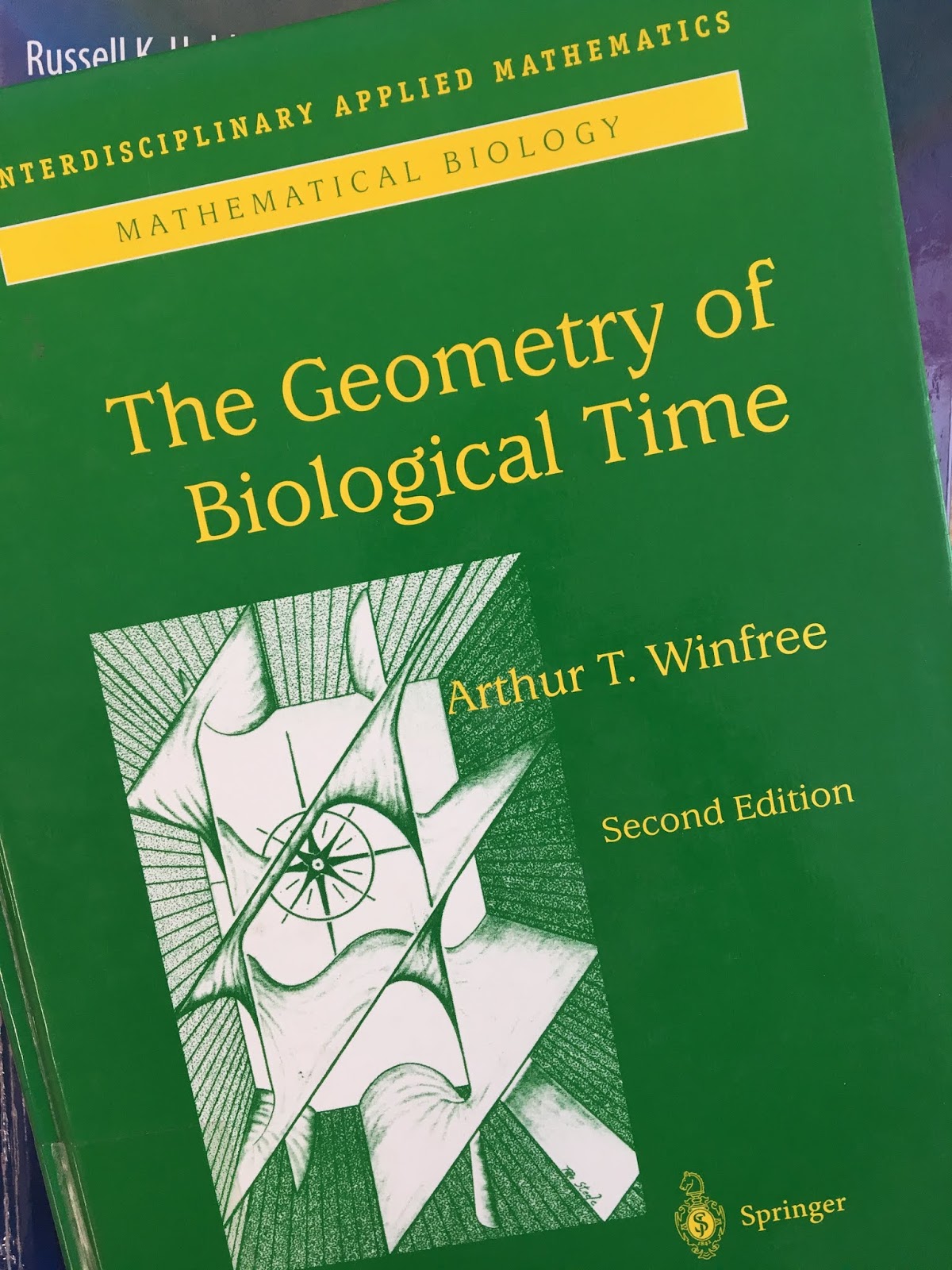 |
| The Geometry of Biological Time, by Art Winfree. |
I walked across the street to Heffer’s Bookstore to browse the books on biomathematics… As I scanned the shelves, with my head tilting sideways, one title popped out at me: The Geometry of Biological Time. Now that was a weird coincidence. My senior thesis on DNA had been subtitled “An Essay on Geometric Biology.” I thought I had invented that odd juxtaposition, geometry next to biology. But the book’s author, someone named Arthur T. Winfree, from the biology department at Purdue University, had obviously connected them first.Strogatz then relates how he corresponded with Winfree, and ended up working with him at Purdue in the summer of 1982. He quotes Winfree’s letters, often written in what Strogatz calls “idiosyncratic code.” This characteristic style brought back memories of my own correspondence with Winfree. Although we only met in person once, I recall us exchanging many emails about cardiac dynamics, with his emails all in that same idiosyncratic code. As I read Winfree’s letters to Strogatz, I found myself thinking “yes, that is exactly the way Winfree would have said it.”
 |
| When Time Breaks Down, by Art Winfree. |
Strogatz describes Winfree’s untimely death in the epilog of Sync.
Tragically, Art Winfree died on November 5, 2002, at age 60, seven months after being diagnosed with brain cancer. He helped me with this book at every stage, even when he was conscious only for a few hours a day. Though he did not live to see it published, he knew that it would be dedicated to him.For more about Winfree’s career, see his website (still available through the University of Arizona), the obituary Strogatz wrote for the Society for Industrial and Applied Mathematics, another by Leon Glass in Nature, and also one in the New York Times.
I described my own interactions with Winfree, and some of his contributions to cardiac electrophysiology, in my paper “Art Winfree and the Bidomain Model of Cardiac Tissue,” published in a special issue of the Journal of Theoretical Biology dedicated to his memory (Volume 230, Pages 445–449, 2004). Other particularly interesting contributions to that issue, full of delightful Winfree anecdotes, were the article by his daughter Rachael, and the article by George Oster.
I thoroughly enjoyed Sync. It is a fine introduction to the mathematics of synchronization and nonlinear dynamics. (Don’t, however, consult the book to learn how lasers work!) Sync ends with a lovely paragraph that explains what motivates scientists:
For reasons I wish I understood, the spectacle of sync strikes a chord in us, somewhere deep in our souls. It’s a wonderful and terrifying thing. Unlike many other phenomena, the witnessing of it touches people at a primal level. Maybe we instinctively realize that if we ever find the source of spontaneous order, we will have discovered the secret of the universe.Alas, my to-do list never gets any shorter. Strogatz has a new book coming out next month, The Calculus of Friendship: What a Teacher and a Student Learned about Life while Corresponding about Math, and I plan to read it as soon as I get a bit of spare time.
Friday, June 26, 2009
Physics Meets Biology
Readers of the 4th edition of Intermediate Physics for Medicine and Biology may find a news feature by Jonathan Knight published in the September 19, 2002 issue of Nature interesting. The article “Physics Meets Biology: Bridging the Culture Gap” (Volume 419, Page 244–246) begins
“In late July, several dozen physicists with an interest in biology gathered at the Colorado mountain resort of Snowmass for a birthday celebration. Hans Frauenfelder, a physicist who began studying proteins decades ago, turned 80 this year. But unofficially, the physicists were celebrating something else—a growing feeling that their discipline’s mindset will be crucial to reaping the harvest of biology’s postgenomic era.It continues:
“Biology today is where physics was at the beginning of the twentieth century,” observes José Onuchic, who is the co-director of the new Center for Theoretical Biological Physics (CTBP) at the University of California, San Diego. “It is faced with a lot of facts that need an explanation.”The article concludes
Physicists believe that they can help, bringing a strong background in theory and the modeling of complexity to nudge the study of molecules and cells in a fresh direction. “What has been all too rare in biology is the symbiosis between theory and experiment that is routine in physics,” says Laura Garwin, director of research affairs at Harvard University’s Bauer Center for Genomics Research, who has made her own transition to biology—she was once Nature’s physical-sciences editor.
“Onuchic believes that immersing young physicists in the culture of biology is the key. At the CTBP, postdocs train in both disciplines simultaneously, developing projects that involve two labs, one in biology and one in physics. They attend two sets of group meetings, and so learn the language and mentality of both disciplines at the same time. “They get inside the culture of the two fields,” Onuchic says. “They get comfortable with the vocabulary and the journals. Life in both labs is more important than any classes you can take.”
Time will tell whether the new generation of biological physicists avoid becoming the lonely children of biology. But for now, the prospects look bright. “We have always been the odd kids in the playground,” says Onuchic. “But we never gave up, and now we are becoming very popular.”
Friday, June 19, 2009
Resource Letter PFBi-1: Physical Frontiers in Biology
Eugenie Mielczarek of George Mason University published “Resource Letter PFBi-1: Physical Frontiers in Biology” in the American Journal of Physics (Volume 74, Pages 375–381, 2006). The fourth edition of Intermediate Physics for Medicine and Biology was one of 39 books listed in the letter.
What are Resource Letters? They are collections of references that are published periodically by the American Journal of Physics.
Readers who enjoy Intermediate Physics for Medicine and Biology will probably find Mielczarek's Resource Letter to be a valuable... well, resource. They may also enjoy her book Iron, Nature's Universal Element: Why People Need Iron and Animals Make Magnets.
Resource Letters are guides for college and university physicists, astronomers, and other scientists to literature, websites, and other teaching aids. Each Resource Letter focuses on a particular topic and is intended to help teachers improve course content in a specific field of physics or to introduce nonspecialists to this field.Mielczarek’s Resource Letter discusses topics that will be of interest to readers of Intermediate Physics for Medicine and Biology.
This Resource Letter provides a guide to the literature on physical frontiers in biology. Books and review articles are cited as well as journal articles for the following topics: cells and cellular mats; conformational dynamics/folding; electrostatics; enzymes, proteins, and molecular machines; material-biomineralization; miscellaneous topics; nanoparticles and nanobiotechnology; neuroscience; photosynthesis; quantum mechanics theory; scale and energy; spectroscopy and microscopy: experiments and instrumentation; single-molecule dynamics; and water and hydrogen-bonded solvents. A list of web resources and videotapes is also given.The letter begins with a fascinating 3-page overview of the role of physics in biology. For instance, Mielczarek asks the question
Which principles govern life? Dutifully the physicist might answer—the organizing of electrons into their lowest energy states, forcing molecules and groups of molecules into specific configurations. But be cautious: this simplistic answer implies an isolated system in equilibrium. It conceals the dynamics of life, which require a continuous input of matter and energy. Cells, tissues and organisms are dependent upon energy refreshment.
 |
| Iron, Nature's Universal Element: Why People Need Iron and Animals Make Magnets, by Eugenie Mielczarek. |
Friday, June 12, 2009
The Magnetic Field of a Single Axon
When I was in graduate school, working in John Wikswo’s lab at Vanderbilt University, I calculated and measured the magnetic field of a single nerve axon. The calculation makes a nice, although slightly advanced, homework problem for Chapter 8 of the 4th edition of Intermediate Physics for Medicine and Biology.
I recall the day I derived this expression for the magnetic field. I was puzzled because another graduate student in Wikswo's lab, James Woosley, had derived a different expression for the magnetic field of an axon using the Biot-Savart law (Sec. 8.2.3). How could there be two seemingly different expressions for the magnetic field? Previous discussions with Prof. John Barach had given me a hint. He had derived two expressions for the magnetic field produced by a battery in a bucket of saline, using either Ampere’s law or the Biot-Savart law, and showed that they were the same (he eventually published this in “The Effect of Ohmic Return Current on Biomagnetic Fields”, Journal of Theoretical Biology, Volume 125, Pages 187–191, 1987). I worried about this problem for some time, until one evening (September 22, 1983; Wikswo insisted that I keep careful records in my lab notebook) I was working on my electricity and magnetism homework and found the solution staring at me: Eq. 3.147 in Jackson’s famous textbook Classical Electrodynamics (here I quote the current 3rd Edition, but at the time I was using my now tattered 2nd Edition with the red cover). This equation defines the Wronskian condition for Bessel functions
I didn't have all my work at home, so I remember riding my bike (I didn’t yet own a car) back to the lab in the rain so I could check if the Wronskian would resolve the difference between my expression and Woosley’s. It did; the two expressions were equivalent (in my usually dry notebook, I wrote “HA! It works”). You can calculate the magnetic field using either Ampere’s law or the Biot-Savart law, and you get the same result. To see how these two equations predict the same magnetic field in a slightly easier case (like that considered by Barach), solve Problem 13 of Chapter 8 in the 4th edition of Intermediate Physics for Medicine and Biology.
For those of you interested in Woosley’s expression, you can find its derivation in “The Magnetic Field of a Single Axon: A Volume Conductor Model” (Woosley, Roth, and Wikswo, Mathematical Biosciences, Volume 76, Pages 1–36, 1985). In particular, they state on page 13
Section 8.2
Problem 14.5 Use Ampere’s law to calculate the magnetic field produced by a nerve axon.
(a) First, solve Problem 30 of Chapter 7 to obtain the electrical potential inside (Vi) and outside (Vo) an axon. The solution will be in terms of the modified Bessel functions I0(kr) and K0(kr), where k is a spatial frequency and r is the radial distance from the center of the axon. Assume the axon has a radius a.
(b) Find the axial component of the current density, J, both inside and outside the axon using Jiz = − σi dVi/dz and Joz = − σo dVo/dz, where σi and σo are the intracellular and extracellular conductivities (Eqs. 6.16b and 6.26).
(c) Integrate Jiz over the axon cross-section to get the total intracellular current. Then integrate Joz over an annulus from a to the radius r, to get the “return current.”
(d) Use Ampere’s law (Eq. 8.9) to calculate the magnetic field. Take the line integral of Ampere's law as a closed loop of radius r concentric with the axon (r greater than a). The current enclosed by this loop is simply the sum of the intracellular and return currents calculated in (c).
In part (c), you will need the Bessel function integrals
To check your solution, see Eq. A13 of “The Magnetic Field of a Single Axon” (Roth and Wikswo, Biophysical Journal, Volume 48, Pages 93–109, 1985). However, that paper uses complex exponentials whereas Problem 30 of Chapter 7 uses sines and cosines, introducing a slight difference between your expression and that in Eq. A13 of the Roth and Wikswo paper.∫ I0(x) x dx = x I1(x)
∫ K0(x) x dx = - x K1(x) .
 |
| Classical Electrodynamics, by John David Jackson. |
I0(x) K1(x) + K0(x) I1(x) = 1/x .
I didn't have all my work at home, so I remember riding my bike (I didn’t yet own a car) back to the lab in the rain so I could check if the Wronskian would resolve the difference between my expression and Woosley’s. It did; the two expressions were equivalent (in my usually dry notebook, I wrote “HA! It works”). You can calculate the magnetic field using either Ampere’s law or the Biot-Savart law, and you get the same result. To see how these two equations predict the same magnetic field in a slightly easier case (like that considered by Barach), solve Problem 13 of Chapter 8 in the 4th edition of Intermediate Physics for Medicine and Biology.
For those of you interested in Woosley’s expression, you can find its derivation in “The Magnetic Field of a Single Axon: A Volume Conductor Model” (Woosley, Roth, and Wikswo, Mathematical Biosciences, Volume 76, Pages 1–36, 1985). In particular, they state on page 13
If we... rearrange terms, and use a relation which can be derived from the Wronskian... we can show that... Equation (45), derived from Ampere’s law, is identical to... Equation (36), derived from the law of Biot and Savart.
 |
| Vanderbilt Research Notebook 4, Page 21, September 22, 1983. |
Friday, June 5, 2009
Ichiji Tasaki (1910-2009)
Ichiji Tasaki (1910–2009) died January 4 in Bethesda, Maryland. Tasaki was known for his discovery in 1939 of saltatory conduction of action potentials in a myelinated nerve axon. You can learn more about myelinated fibers and saltatory conduction in the 4th edition of Intermediate Physics for Medicine and Biology.
Tasaki had a long and fascinating career in science. His life is described in an obituary published in the May 2009 issue of Neuroscience Research. He is also featured in an article of the NIH Record, the weekly newsletter for employees of the National Institutes of Health.
I knew Tasaki when I was working at NIH in the 1990s. Late in his career he worked with my friend Peter Basser in the National Institute of Child Health and Human Development. I recall him working every day in his laboratory, despite being in his 80s, with his wife as his assistant. He led a fascinating life. His best known research on saltatory conduction was performed in Japan just before and during World War II. After the war, he spent over 50 years at NIH.
Basser describes Tasaki as “a scientist’s scientist, never afraid to question current dogma, always digging deeper to discover the truth.” Congressman Chris van Hollen of Maryland paid tribute to Tasaki a few months before he died, beginning “Madam Speaker, I rise today to recognize the outstanding achievements of my constituent Dr. Ichiji Tasaki. Dr. Tasaki has worked at the National Institutes of Health for 54 years, since November 1953, and has made invaluable contributions to the scientific community.”
Friday, May 29, 2009
Deep Brain Stimulation
In Chapter 7 of the 4th edition of Intermediate Physics for Medicine and Biology, Russ Hobbie and I describe electrical stimulation (Section 7.10, pages 192–196), including excitation of peripheral nerves (Problems 7.38–7.41) and cardiac pacemakers. Another increasingly important procedure is deep brain stimulation. On May 21, Medtronic announced Food and Drug Administration approval of two new models of the Activa stimulator for use in the United States to treat Parkinson’s disease and essential tremor. This device is similar to a pacemaker, but electrodes are implanted in the brain instead of the heart. The detailed electrophysiological mechanism is still unknown, but repetitive stimulation of certain structures deep in the brain provides dramatic relief to some patients with movement disorders. The new Activa RC and PC stimulators have features not available in older models, such as the RC’s rechargeable battery.
A friend of mine, Frans Gielen, has worked on deep brain stimulation at the Medtronic Bakken Research Centre in Maastricht, the Netherlands. Frans was a post doc when I was a graduate student at Vanderbilt University, working in the laboratory of John Wikswo; we both worked on measuring the magnetic field of nerves and muscle fibers (for instance, see Gielen, Roth and Wikswo, “Capabilities of a Toroid-Amplifier System for Magnetic Measurement of Current in Biological Tissue,” IEEE Transactions on Biomedical Engineering, Volume 33, Pages 910–921, 1986). Frans is considered at Medtronic as “the architect of the Medtronic Activa Tremor Control Therapy.” Known fondly while in Wikswo’s lab as “that crazy Dutchman,” when he left Vanderbilt we were not surprised that Frans would make important contributions to Medtronic.
For more about deep brain stimulation, two review articles are “Deep Brain Stimulation for Parkinson's Disease” (Benabid AL, Current Opinion in Neurobiology, Volume 13, Pages 696–706 2003) and “Uncovering the Mechanism(s) of Action of Deep Brain Stimulation: Activation, Inhibition, or Both” (McIntyre CC, Savasta M, Kerkerian-Le Goff L, Vitek JL, Clinical Neurophysiology, Volume 115, Pages 1239–1248, 2004).
For those wanting to read about deep brain stimulation from the patient's perspective, see Deep Brain Stimulation: A New Treatment Shows Promise in the Most Difficult Cases, by Jamie Talan. In the Prologue, Talan writes
A friend of mine, Frans Gielen, has worked on deep brain stimulation at the Medtronic Bakken Research Centre in Maastricht, the Netherlands. Frans was a post doc when I was a graduate student at Vanderbilt University, working in the laboratory of John Wikswo; we both worked on measuring the magnetic field of nerves and muscle fibers (for instance, see Gielen, Roth and Wikswo, “Capabilities of a Toroid-Amplifier System for Magnetic Measurement of Current in Biological Tissue,” IEEE Transactions on Biomedical Engineering, Volume 33, Pages 910–921, 1986). Frans is considered at Medtronic as “the architect of the Medtronic Activa Tremor Control Therapy.” Known fondly while in Wikswo’s lab as “that crazy Dutchman,” when he left Vanderbilt we were not surprised that Frans would make important contributions to Medtronic.
For more about deep brain stimulation, two review articles are “Deep Brain Stimulation for Parkinson's Disease” (Benabid AL, Current Opinion in Neurobiology, Volume 13, Pages 696–706 2003) and “Uncovering the Mechanism(s) of Action of Deep Brain Stimulation: Activation, Inhibition, or Both” (McIntyre CC, Savasta M, Kerkerian-Le Goff L, Vitek JL, Clinical Neurophysiology, Volume 115, Pages 1239–1248, 2004).
 |
| Deep Brain Stimlation, by Jamie Talan. |
On March 14, 1997, the U.S. Food and Drug Administration held a hearing on the use of deep brain stimulation (DBS) as a treatment for essential tremor and Parkinson’s disease. By that time, excitement about this technology, which could restore a body to its rightful state of controlled movement, had spread through brain research laboratories and neurology clinics around the world. Desperate patients with all kinds of movement disorders had heard about deep brain stimulation, too, and they were clamoring for access to the treatment.
On this day in March, two American patients, Maurice Long and George Shafer, were standing before an advisory panel commissioned by the FDA to study the benefits and risks of deep brain stimulation. Long and Shafer were among the 83 people with essential tremor and 113 people with Parkinson's tremor who had undergone deep brain stimulation in a large clinical trial. The FDA-approved study was sponsored by Medtronic, the Minneapolis-based company that supplied the simulating electrodes for the trial. Founded in 1949 to usher in a new technology called cardiac pacing, Medtronic had made the first implantable heart pacemaker. Now the company was in the middle of an international push on another frontier: the brain seemed to be as receptive to electrical stimulation as the heart.
Friday, May 22, 2009
Using Logarithmic Transformations When Fitting Allometric Data
In the 4th edition of Intermediate Physics for Medicine and Biology, Russ Hobbie and I discuss least squares fitting. A homework problem at the end of Chapter 11 (see page 321) asks the student to fit some data to a power law.
However, inquisitive students may ask “what if I don’t follow the hint, and do a least squares fit to the original power law without taking logarithms. Do I get the same result?” This becomes a more difficult problem, since you must now make a nonlinear least squares fit. Nevertheless, I solved the problem this way (using a terribly inefficient iterative guess-and-check method) and found R = 0.0619 M0.358.
Which solution is correct? Gary Packard and Thomas Boardman, both from Colorado State University, address this question in their paper “A Comparison of Methods for Fitting Allometric Equations to Field Metabolic Rates of Animals” (Journal of Comparative Physiology, B, Volume 179, Pages 175–182, 2009), and find that
Packard and Boardman make a persuasive case that you might want to ignore our hint at the end of Problem 11. However, if you do ignore it, you had better be prepared to do nonlinear least squares fitting. See Sec. 11.2, Nonlinear Least Squares, in our book to get started.
For more about this subject, see Packard’s letter to the editor in the Journal of Theoretical Biology (Volume 257, Pages 515–518, 2009). Also, Russ Hobbie has a paper submitted to the journal Ecology that discusses a similar issue with exponential, rather than power law, least squares fits (“Single pool exponential decomposition models: Potential pitfalls in their use in ecological studies”). Russ’s coatuhors are E. Carol Adair and Sarah E. Hobbie (Russ’s daughter), both of the University of Minnesota in Saint Paul.
Problem 11 Consider the data given in Problem 2.36 relating molecular weight M and molecular radius R. Assume the radius is determined from the molecular weight by a power law: R = B Mn. Fit the data to this expression to determine B and n. Hint: Take logarithms of both sides of the equation.The solution manual (available at the book’s website, contact one of the authors for the password) outlines how taking logarithms makes the problem linear, so a simple linear least squares fit gives the solution R = 0.0534 M0.371.
However, inquisitive students may ask “what if I don’t follow the hint, and do a least squares fit to the original power law without taking logarithms. Do I get the same result?” This becomes a more difficult problem, since you must now make a nonlinear least squares fit. Nevertheless, I solved the problem this way (using a terribly inefficient iterative guess-and-check method) and found R = 0.0619 M0.358.
Which solution is correct? Gary Packard and Thomas Boardman, both from Colorado State University, address this question in their paper “A Comparison of Methods for Fitting Allometric Equations to Field Metabolic Rates of Animals” (Journal of Comparative Physiology, B, Volume 179, Pages 175–182, 2009), and find that
the discrepancies could be caused by four sources of bias acting singly or in combination to cause exponents (and coefficients) estimated by back-transformation from logarithms to be inaccurate and misleading. First, influential outliers may go undetected in some analyses ... owing to the altered relationship between X and Y variables that accompanies logarithmic transformation ... Second, the use of logarithmic transformations may result in the fitting of mathematical functions (i.e., two-parameter power functions) that are poor descriptors of data in the original scale ... Third, a two-parameter power function ... fitted to the original data by least squares invokes a statistical model with additive error Y = aXb + e and predicts arithmetic means for Y whereas a straight line fitted to logarithmic transformations of the data by least squares invokes an underlying model with multiplicative error Y = aXb 10e and predicts geometric means for the response variable ... And fourth, linear regression on nonlinear transformations like logarithms may introduce further bias into analyses by the unequal weighting of large and small values for both X and Y...Their paper concludes
Conversion to logs results in an overall compression of the distributions for both the Y- and X-variables, but the compression is greater at the high ends of the scales than at the low ends... Consequently, linear regression on transformations gives unduly large influence to small values for Y and X and unduly small influence to large ones... This disparate influence is apparent in plots of back-transformations against the backdrop of data in their original scales, where the location of data for the largest animals had little apparent influence on fits of the lines.
Why transform? Log transformations have a long history of use in allometric research... and have been justified on grounds ranging from linearizing data to achieving better distributions for purposes of graphical display... However, most of the reasons for making such transformations disappeared with the advent of powerful PCs and sophisticated software for graphics and statistics. Indeed, the only ongoing application for log transformations in allometric research is in adjusting (‘‘stabilizing’’) distributions when residuals from analyses performed in the original scale are not distributed normally and/or when variances are not constant at all values for X. Assuming that log transformations actually linearize the data and produce the desired distributions, the regression of log Y on log X will yield evidence for a dependency between Y and X values in their original state, and statistical comparisons can be made with other samples that also are expressed in logarithmic form. However, interpretations about patterns of variation of the variables in the arithmetic domain seldom are warranted... because transformation fundamentally alters the relationship between the predictor and response variables. Interest typically is in patterns of variation of data expressed in an arithmetic scale, so this is the scale in which allometric analyses need to be performed if it is at all possible to do so.In the above quote, many of the “...”s indicate important references that I skipped to save space.
Implications for allometric research. Accumulating evidence from the field of biology... and beyond... gives cause for concern about the accuracy and reliability of allometric equations that have been estimated in the traditional way... This concern has special bearing on the current debate about the “true’’ exponent for scaling of metabolism to body mass because exponents of 2/3 and 3/4 need both to be viewed with some skepticism. The aforementioned evidence also indicates that the traditional approach to allometric analysis may need to be abandoned in favor of a new research paradigm that will prevent future studies from being compromised by the insidious effects of logarithmic transformations.
Packard and Boardman make a persuasive case that you might want to ignore our hint at the end of Problem 11. However, if you do ignore it, you had better be prepared to do nonlinear least squares fitting. See Sec. 11.2, Nonlinear Least Squares, in our book to get started.
For more about this subject, see Packard’s letter to the editor in the Journal of Theoretical Biology (Volume 257, Pages 515–518, 2009). Also, Russ Hobbie has a paper submitted to the journal Ecology that discusses a similar issue with exponential, rather than power law, least squares fits (“Single pool exponential decomposition models: Potential pitfalls in their use in ecological studies”). Russ’s coatuhors are E. Carol Adair and Sarah E. Hobbie (Russ’s daughter), both of the University of Minnesota in Saint Paul.
Subscribe to:
Posts (Atom)

