The Atomic Energy Merit Badge

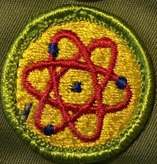
My Atomic Energy Merit Badge.

Chapter 17 of Intermediate Physics for Medicine and Biology discusses nuclear physics and nuclear medicine. I began studying nuclear physics fifty years ago. It all started in the Boy Scouts.

Troop 96, Morrison, Illinois.

When growing up in Morrison, Illinois, I was a member of the Cub Scouts and then the Boy Scouts. I enjoyed the camping, hiking, and canoeing. Each summer I spent a week at scout camp, and loved it. In the winter, we would have a Klondike Derby, which involved pushing a large sled over the snow and then camping in the cold. I was a member of Morrison’s Troop 96 and Mr. Glenn Van Eaton was our Scoutmaster; behind his back we called him “General Glenn.” One of my fondest memories was being inducted into the Order of the Arrow. At a campfire ceremony, several of us were “tapped-out” for initiation, which involved spending a night in the woods alone.

My Scout Handbook.

Between campouts, we earned merit badges. Some of them you'd expect, such as first-aid, rowing, swimming, and pioneering (knot tying). Others examined adult topics, such as atomic energy.

I found my old Scout Handbook—molding in a box in our basement—and looked up the requirements for the atomic energy merit badge. They are impressive. Completing this merit badge provides a good preparation for Chapter 17 of IPMB.

1. Tell the meaning of the following: alpha particle, atom, background radiation, beta particle, curie, fallout, half-life, ionization, isotope, neutron activation, nuclear reactor, particle accelerator, radiation, radioactivity, roentgen, and X-ray. 
2. Make three-dimensional models of the atoms of the three isotopes of hydrogen. Show neutrons, protons, and electrons. Use these models to explain the difference between atomic weight and number. 
3. Make a drawing showing how nuclear fission happens. Label all details. Draw a second picture showing how a chain reaction could be started. Also show how it could be stopped. Show what is meant by “critical mass.”
4. Tell who five of the following people were. Explain what each of the five discovered in the field of atomic energy: Henri Becquerel, Niels Bohr, Marie Curie, Albert Einstein, Enrico Fermi, Otto Hahn, Ernest Lawrence, Lise Meitner, William Rontgen, and Sir Ernest Rutherford. Explain how any one person’s discovery was related to one other person’s work. 
5. Draw and color the radiation hazard symbol. Explain where it should be used and not used. Tell why and how people must use radiation or radioactive materials carefully.
6. Do any THREE of the following:
   1. Build an electroscope. Show how it works. Put a radiation source inside it. Explain any difference seen. 
   2. Make a simple Geiger counter. Tell the parts. Tell which types of radiation the counter can spot. Tell how many counts per minute of what radiation you have found in your home. 
   3. Build a model of a reactor. Show the fuel, the control rods, the shielding, the moderator, and any cooling material. Explain how a reactor could be used to change nuclear into electrical energy or make things radioactive. 
   4. Use a Geiger counter and a radiation source. Show how the counts per minute change as the source gets closer. Put three different kinds of material between the source and the detector. Explain any differences in the counts per minute. Tell which is the best to shield people from radiation and why. 
   5. Use fast-speed film and a radiation source. Show the principles of autoradiography and radiography. Explain what happened to the films. Tell how someone could use this in medicine, research, or industry. 
   6. Using a Geiger counter (that you have built or borrowed), find a radiation source that has been hidden under a covering. Find it in at least three other places under the cover. Explain how someone could use this in medicine, research, agriculture, or industry. 
   7. Visit a place where X-rays are used. Draw a floor plan of the room in which it is used. Show where the unit is. Show where the unit, the person who runs it, and the patient would be when it is used. Describe the radiation dangers from X-rays. 
   8. Make a cloud chamber. Show how it can be used to see the tracks caused by radiation. Explain what is happening. 
   9. Visit a place where radioisotopes are being used. Explain by a drawing how and why they are used. 
   10. Get samples of irradiated seeds. Plant them. Plant a group of nonirradiated seeds of the same kind. Grow both groups. List any differences. Discuss what irradiation does to seeds.

Build a Geiger counter? Mom would have vetoed that!

Working on the atomic energy merit badge may have been my initial exposure to physics; the first step in a long journey. Now it is called the nuclear science merit badge. Some of the requirements are the same, but there is more emphasis on radiation hazards (for example, radon) and nuclear medicine. Probably it is even better at preparing you for Intermediate Physics for Medicine and Biology.

My dad made it to Eagle Scout when he was young, but I didn’t uphold the family tradition. I quit scouts with the rank of Life. Most boys enter high school and lose interest in scouting, but a few hang on and make it to Eagle. I was planning on being one of the few, but when we moved out of town after my sophomore year I didn't restart with a new troop. Besides, I attended high school in the post-Vietnam/Watergate era, when scouting went out of fashion. Over the years, I came to disagree with the Boy Scouts’ positions on homosexuality and religion, so I don’t regret dropping out. But when I was a kid in Morrison, those issues never came up. We just had fun.

My Order of the Arrow sash.

My 18 merit badges (left to right, then top to bottom):
Stamp Collecting, First Aid, Music,
Swimming, Cooking, Canoeing,
Rowing, Camping, Reading,
Citizenship in the Nation, Emergency Preparedness, Citizenship in the Community,
Citizenship in the World, Atomic Energy, Scholarship,
Fish and Wildlife Management, Pioneering, and Environmental Science.
Those with a silver rim are required for Eagle.

Sunscreen

In Chapter 14 of Intermediate Physics for Medicine and Biology, Russ Hobbie and I discuss ultraviolet light, and specifically sunscreen.

Protection from the sun certainly reduces erythema [sunburn] and probably reduces skin cancer. Protection is most important in childhood years, both because children receive three times the annual sun exposure of adults and because the skin of children is more susceptible to cancer-causing changes. The simple sun protection factor (SPF) alone is not an adequate measure of effectiveness, because it is based on erythema, which is caused mainly by UVB [ultraviolet B light, with wavelengths from 280 to 315 nm]. Some sunscreens do not adequately protect against UVA radiation [315-400 nm]. Buka (2004) reviews both sunscreens and insect repellents for children. He finds several products that adequately block both UVA and UVB. Look for a sunscreen labeled “broad spectrum” or with at least three stars in a UVA rating system. An adequate amount must be used: for children he recommends 1 fluid ounce (30 ml) per application of a product with SPF of 15 or more. The desired application of sunscreen is 2 mg cm⁻². Typical applications are about half this amount. It has been suggested that one make two applications (Teramura et al.2012) or use a sunscreen with a very high SPF (Hao et al.2012).

This week the Food and Drug Administration has issued a proposed update to sunscreen rules.

This significant action is aimed at bringing nonprescription, over-the-counter (OTC) sunscreens that are marketed without FDA-approved applications up to date with the latest science to better ensure consumers have access to safe and effective preventative sun care options. Among its provisions, the proposal addresses sunscreen active ingredient safety, dosage forms, and sun protection factor (SPF) and broad-spectrum requirements. It also proposes updates to how products are labeled to make it easier for consumers to identify key product information.

“Broad spectrum sunscreens with SPF values of at least 15 are critical to the arsenal of tools for preventing skin cancer and protecting the skin from damage caused by the sun’s rays, yet some of the essential requirements for these preventive tools haven’t been updated in decades. Since the initial evaluation of these products, we know much more about the effects of the sun and about sunscreen’s absorption through the skin. Sunscreen usage has changed, with more people using these products more frequently and in larger amounts. At the same time, sunscreen formulations have evolved as companies innovated. Today’s action is an important step in the FDA’s ongoing efforts to take into account modern science to ensure the safety and effectiveness of sunscreens,” said FDA Commissioner Scott Gottlieb, M.D. “The proposal we’ve put forward would improve quality, safety and efficacy of the sunscreens Americans use every day. We will continue to work with industry, consumers and public health stakeholders to ensure that we’re striking the right balance. To further advance these goals, we’re also working toward comprehensive OTC reform, which will help foster OTC product innovation as well as facilitate changes necessary for the FDA to keep pace with evolving science and new safety data.”

The agency is issuing this proposed rule to put into effect final monograph regulations for OTC sunscreen drug products as required by the Sunscreen Innovation Act. OTC monographs establish conditions under which the FDA permits certain OTC drugs to be marketed without approved new drug applications because they are generally recognized as safe and effective (GRASE) and not misbranded. Over the last twenty years, new scientific evidence has helped to shape the FDA’s perspective on the conditions, including active ingredients and dosage forms, under which sunscreens could be considered GRASE.

The feds then get specific.

Of the 16 currently marketed active ingredients, two ingredients – zinc oxide and titanium dioxide – are GRASE for use in sunscreens; two ingredients – PABA and trolamine salicylate – are not GRASE for use in sunscreens due to safety issues. There are 12 ingredients for which there are insufficient safety data to make a positive GRASE determination at this time.

Latha et al. (Sunscreening Agents: A Review, The Journal of Clinical and Aesthetic Dermatology, Volume 6, Pages 16-26, 2013) discuss the mechanism of sunscreen action (references removed).

Sunscreening agents contain titanium dioxide (TiO₂), kaolin, talc, zinc oxide (ZnO), calcium carbonate, and magnesium oxide. Newer chemical compounds, such as bemotrizinol, avobenzone, bisoctizole [sic], benzophenone-3 (BZ-3, oxybenzone), and octocrylene, are broad-spectrum agents and are effective against a broad range of solar spectrum both in experimental models and outdoor settings. Ecamsule (terephthalylidene dicamphor sulphonic acid), dometrizole trisiloxane [sic], bemotrizinol, and bisoctrizole are considered organic UVA sunscreening agents... Commercial preparations available in the market include a combination of these agents to cover a wide range of UV rays.

Composition and mechanism of action of sunscreening agents vary from exerting their action through blocking, reflecting, and scattering sunlight. Chemical sunscreens absorb high-energy UV rays, and physical blockers reflect or scatter light. Multiple organic compounds are usually incorporated into chemical sunscreening agents to achieve protection against a range of the UV spectrum. Inorganic particulates may scatter the microparticles in the upper layers of skin, thereby increasing the optical pathway of photons, leading to absorption of more photons and enhancing the sun protection factor (SPF), resulting in high efficiency of the compound.

Researchers are postulating that the generation of sunlight-induced free radicals causes changes in skin; use of sunscreens reduces these free radicals on the skin, suggesting the antioxidant property. Broad-spectrum agents have been found to prevent UVA radiation-induced gene expression in vitro in reconstructed skin and in human skin in vivo.

Sunscreens may have unanticipated side effects. For instance, Key West banned sunscreens containing oxybenzone and octinoxate, two chemicals that damage coral reefs.

Do sunscreens cause cancer? Read what Harriet Hall, the SkepDoc, thinks (quick summary: no).

To learn more about sunscreens, here’s a video from one of my favorite explainers of physics: Dianna Cowern, The Physics Girl. She’s GRASE.

Happy physicsing!

Dianna Cowern, The Physics Girl, discussing sunscreens.

Francis Crick, Biological Physicist

I'm fascinated by scientists who straddle physics and biology. In particular, I'm curious how a scientist trained in one field switches to another. The quintessential physicist-turned-biologist is Francis Crick. Yes, I mean Crick of “Watson and Crick," the team who discovered the structure of DNA.

Asimov's Biographical
Encyclopedia of Science
and Technology

To start learning about the education of Francis Crick, consider his entry in Asimov’s Biographical Encyclopedia of Science and Technology.

CRICK, Francis Harry Compton

English biochemist

Born: Northampton, June 8, 1916

Crick was educated at University College in London and went on to obtain his Ph.D. at Cambridge University in 1953. He was a physicist to begin with and worked in the field during World War II, when he was involved in radar research and in magnetic mine development…

At the time, under the leadership of [Max] Perutz, a veritable galaxy of physics-minded scientists was turning to biochemistry at Cambridge and their refined probings established the science of molecular biology, as fusion of biology, chemistry, and physics…

Crick was one of the physicists who turned to biochemistry or, rather, to molecular biology, and with him was a young American, James Dewey Watson…

The Eighth Day of Creation,
by Horace Freeland Judson.

To explore in more detail how Crick changed from physics to biology, let’s turn to the definitive history of modern biology: Horace Freeland Judson’s masterpiece The Eighth Day of Creation.

Crick is to an unusual extent self-educated in biology. He went to a minor English public school, Mill Hill, in northern London; his interest in science was already so single-minded that his family thought him odd. At University College, London, he read physics and had nearly finished his doctorate when the war broke out and a German bomb destroyed his laboratory and gear. When Crick left the Admiralty and physics in 1947, he set out to master the literature of biology, reading with an appetite that has slackened, if at all, only in the last few years [Judson published The Eighth Day of Creation in 1979]. His peers concede without question his astonishing reach. Perutz, whose knowledge is encyclopedic in scope and order: “Francis of course reads more widely than the rest of us.” Jacques Monod, the science’s other great theorist: “No one man discovered or created molecular biology. But one man dominates intellectually the whole field, because he knows the most and understands the most. Francis Crick.”

This idea that you have to read the literature resonates with me. I spent the first months of graduate school at Vanderbilt reading research articles about how nerves worked. I took no classes in neurobiology. I didn’t have a biological mentor (my PhD advisor, John Wikswo, was a physicist). I just read. That's the way many physicists learn biology.

Judson humorously tells of Crick's introduction to Perutz's laboratory:

"The first thing Francis did was to read everything we had done," Perutz said. "Then he started criticizing."

Why did Crick change to biology? Judson explains

“An important reason Crick changed to biology, he said to me, was that he is an atheist, and was impatient to throw light into the remaining shadowy sanctuaries of vitalistic illusions. ‘I had read [Erwin] Schrodinger’s little book [What is Life?], too [According to Judson, "everyone read Schrodinger."]. Essentially, if you read that book critically, the main import is very peculiar; for one thing, it’s a book written by a physicist who doesn’t know any chemistry! But the impact—there’s no doubt that Schrodinger wrote it in a compelling style, not like the junk that most people write, and it was imaginative. It suggested that biological problems could be thought about, in physical terms—and thus gave the impression that exciting things in this field were not far off. My own motives I never had any doubt about; I was very clear in my mind. Because when I decided to leave the Admiralty, when I was about thirty, then on the grounds that I knew so little anyway I might just as well go into anything I liked, I looked around for fields which would illuminate this particular point of view, against vitalism. And the two fields I chose were what we would now call molecular biology, though the term wasn’t common then, certainly I didn’t know it—but I would have said the borderline between the living and nonliving. That was the phrase I had in my mind, on the one hand. And on the other, the higher nervous system and this problem of consciousness...”

What Mad Pursuit:
A Personal View
of Scientific Discovery,
by Francis Crick.

Crick reminisces about his shift from physics to biology in his autobiography What Mad Pursuit.

"By the time most scientists have reached age thirty they are trapped by their own expertise. They have invested so much effort in one particular field that it is often extremely difficult, at that time in their careers, to make a radical change. I, on the other hand, knew nothing, except for a basic training in somewhat old-fashioned physics and mathematics and an ability to turn my hand to new things. I was sure in my mind that I wanted to do fundamental research rather than going into applied research...

Since I essentially knew nothing, I had an almost completely free choice...Working in the Admiralty, I had several friends among the naval officers. They were interested in science but knew even less about it than I did. One day I noticed that I was telling them, with some enthusiasm, about recent advances in antibiotics—penicillin and such. Only that evening did it occur to me that I myself really knew almost nothing about these topics...It came to me that I was not really telling them about science. I was gossiping about it.

This insight was a revelation to me. I had discovered the gossip test—what you are really interested in is what you gossip about. Without hesitation, I applied it to my recent conversations. Quickly I narrowed down my interests to two main areas: the borderline between the living and nonliving, and the workings of the brain..."

I'm not sure Crick's reflections can be generalized. To me, they imply that the choice of a research topic can be haphazard and personal.

Four good books.

Perhaps more useful is Crick's thoughts about theory in biology, which appear in the conclusion of What Mad Pursuit.

"Physicists are all too apt to look for the wrong sorts of generalizations, to concoct theoretical models that are too neat, too powerful, and too clean. Not surprisingly, these seldom fit well with the data. To produce a really good biological theory one must try to see through the clutter produced by evolution to the basic mechanisms lying beneath them, realizing that they are likely to be overlaid by other, secondary mechanisms. What seems to physicists to be a hopelessly complicated process may have been what nature found simplest, because nature could only build on what was already there...

The job of theorists, especially in biology, is to suggest new experiments. A good theory makes not only predictions, but surprising predictions that then turn out to be true. (If its predictions appear obvious to experimentalists, why would they need a theorist?) ... If this book helps anyone to produce good biological theories, it will have performed one of its main functions."

Crick is a case study into how and why a physicist switches to studying biology. Readers of Intermediate Physics for Medicine and Biology who are contemplating such a switch may benefit from his story.

Want to learn more? Listen to Crick himself discuss how he became interested in science.

 Listen to Francis Crick talking about how he became interested in science.

The Electric Field Induced During Magnetic Stimulation

Chapter 8 of Intermediate Physics for Medicine and Biology discusses electromagnetic induction and magnetic stimulation of nerves. It doesn't, however, explain how to calculate the electric field. You can learn how to do this from my article “The Electric Field Induced During Magnetic Stimulation” (Electroencephalography and Clinical Neurophysiology, Supplement 43, Pages 268-278, 1991). It begins:

“The Electric Field Induced
During Magnetic Stimulation.”

Magnetic stimulation has been studied widely since its use in 1982 for stimulation of peripheral nerves (Polson et al. 1982), and in 1985 for stimulation of the cortex (Barker et al. 1985). The technique consists of inducing current in the body by Faraday’s law of induction: a time-dependent magnetic field produces an electric field. The transient magnetic field is created by discharging a capacitor through a coil held near the target neuron. Magnetic stimulation has potential clinical applications for the diagnosis of central nervous system disorders such as multiple sclerosis, and for monitoring the corticospinal tract during spinal cord surgery (for review, see Hallett and Cohen 1989). When activating the cortex transcranially, magnetic stimulation is less painful than electrical stimulation.

Appendix 1.

Although there have been many clinical studies of magnetic stimulation, until recently there have been few attempts to measure or calculate the electric field distribution induced in tissue. However, knowledge of the electric field is important for determining where stimulation occurs, how localized the stimulated region is, and what the relative efficacy of different coil designs is. In this paper, the electric field induced in tissue during magnetic stimulation is calculated, and results are presented for stimulation of both the peripheral and central nervous systems.

In Appendix 1 of this article, I derived an expression for the electric field E at position r, starting from

where N is the number of turns in the coil, μ₀ is the permeability of free space (4π × 10^-7 H/m), I is the coil current, r' is the position along the coil, and the integral of dl' is over the coil path. For all but the simplest of coil shapes this integral can't be evaluated analytically, so I used a trick: approximate the coil as a polygon. A twelve-sided polygon looks a lot like a circular coil. You can make the approximation even better by using more sides.

A circular coil (black) approximated by
a 12-sided polygon (red).

With this method I needed to calculate the electric field only from line segments. The calculation for one line segment is summarized in Figure 6 of the paper.

Figure 6 from “The Electric Field
Induced During Magnetic Stimulation.”

I will present the calculation as a new homework problem for IPMB. (Warning: t has two meanings in this problem: it denotes time and is also a dimensionless parameter specifying location along the line segment.)

Section 8.7

Problem 32 ½. Calculate the integral

for a line segment extending from x₂ to x₁. Define δ = x₁ - x₂ and R = r - ½(x₁ + x₂).

(a) Interpret δ and R physically.

(b) Define t as a dimensionless parameter ranging from -½ to ½. Show that r' equals r – R – tδ.

(c) Show that the integral becomes

(d) Evaluate this integral. You may need a table of integrals.

(e) Express the integral in terms of δ, R, and φ (the angle between R and δ).

The resulting expression for the electric field is Equation 15 in the article

Equation (15) in “The Electric Field Induced During Magnetic Stimulation.”

The photograph below shows the preliminary result in my research notebook from when I worked at the National Institutes of Health. I didn't save the reams of scrap paper needed to derive this result.

The November 10, 1988 entry
in my research notebook.

To determine the ends of the line segments, I took an x-ray of a coil and digitized points on it. Below are coordinates for a figure-of-eight coil, often used during magnetic stimulation. The method was low-tech and imprecise, but it worked.

The November 17, 1988 entry
in my research notebook.

Ten comments:

• My coauthors were Leo Cohen and Mark Hallett, two neurologists at NIH. I recommend their four-page paper “Magnetism: A New Method for Stimulation of Nerve and Brain.”
• The calculation above gives the electric field in an unbounded, homogeneous tissue. The article also analyzes the effect of tissue boundaries on the electric field.
• The integral is dimensionless. “For distances from the coil that are similar to the coil size, this integral is approximately equal to one, so a rule of thumb for determining the order of magnitude of E is 0.1 N dI/dt, where dI/dt has units of A/μsec and E is in V/m.”
• The inverse hyperbolic sine can be expressed in terms of logarithms: sinh^-1z = ln[z + √(z² + 1)]. If you're uncomfortable with hyperbolic functions, perhaps logarithms are more to your taste. 
  
• This supplement to Electroencephalography and Clinical Neurophysiology contained papers from the International Motor Evoked Potential Symposium, held in Chicago in August 1989. This excellent meeting guided my subsequent research into magnetic stimulation. The supplement was published as a book: Magnetic Motor Stimulation: Principles and Clinical Experience, edited by Walter Levy, Roger Cracco, Tony Barker, and John Rothwell. 
• Leo Cohen was first author on a clinical paper published in the same supplement: Cohen, Bandinelli, Topka, Fuhr, Roth, and Hallett (1991) “Topographic Maps of Human Motor Cortex in Normal and Pathological Conditions: Mirror Movements, Amputations and Spinal Cord Injuries.”
• To be successful in science you must be in the right place at the right time. I was lucky to arrive at NIH as a young physicist in 1988—soon after magnetic stimulation was invented—and to have two neurologists using the new technique on their patients and looking for a collaborator to calculate electric fields.
• A week after deriving the expression for the electric field, I found a similar expression for the magnetic field. It was never published. Let me know if you need it.
• If you look up my article, please forgive the incorrect units for μ₀ given in the Appendix. They should be Henry/meter, not Farad/meter. In my defense, I had it correct in the body of the article. 
• Correspondence about the article was to be sent to “Bradley J. Roth, Building 13, Room 3W13, National Institutes of Health, Bethesda, MD 20892.” This was my office when I worked at the NIH intramural program between 1988 and 1995. I loved working at NIH as part of the Biomedical Engineering and Instrumentation Program, which consisted of physicists, mathematicians and engineers who collaborated with the medical doctors and biologists. Cohen and Hallett had their laboratory in the NIH Clinical Center (Building 10), and were part of the National Institute of Neurological Disorders and Stroke. Hallett once told me he began his undergraduate education as a physics major, but switched to medicine after one of his professors tried to explain how magnetic fields are related to electric fields in special relativity.

A map of the National Institutes of Health campus
in Bethesda, Maryland.

BrainFacts.org

BrainFacts.org

In this blog, I sometimes share websites related to Intermediate Physics for Medicine and Biology. Recently, I discovered BrainFacts.org.

The human brain is the most complex biological structure in the known universe. Its roughly 86 billion nerve cells power all of our thoughts, perceptions, memories, emotions, and actions. It’s what inspires us to build cities and compels us to gaze at the stars.

That sense of wonder drives BrainFacts.org. We are a public information initiative of The Kavli Foundation, the Gatsby Charitable Foundation, and the Society for Neuroscience – global nonprofit organizations dedicated to advancing brain research.

Powered by the global neuroscience community and overseen by an editorial board of leading neuroscientists from around the world, BrainFacts.org shares the stories of scientific discovery and the knowledge they reveal. Unraveling the mysteries of the brain has the potential to impact every aspect of human experience and civilization.

Join us as we explore the universe between our ears. Because when you know your brain, you know yourself.

“To Understand the Brain,
You Have to Do the Math.”

Browsing BrainFacts.org is an excellent way to learn about neuroscience. The articles are beautifully written, with a professional polish honed by a team of talented science writers (unlike hobbieroth.blogspot.com, written by an aging amateur journalist-wannabe; a one-man-band hawking textbooks). My favorite article—one in the spirit of IPMB—is “To Understand the Brain, You Have to Do the Math” by Alexandre Pouget. He concludes

The brain is the most complex computational device we know in the universe…and unless we do the math, unless we use mathematical theories, there’s absolutely no way we’re ever going to make sense of it.

Browsing BrainFacts.org prompted me to examine how useful Intermediate Physics for Medicine and Biology is for students of neuroscience.

• Chapter 6 is about how nerve axons fire action potentials, which is critical for understanding how neurons in the brain communicate with other neurons and with the rest of the body.
• Chapter 7 discusses functional electrical stimulation of nerves, and mentions deep brain stimulation. It also considers electroencephalography, a tool for monitoring brain function.
• Chapter 8 outlines the physics behind magnetoencephalography as well as transcranial magnetic stimulation.
• Chapter 9 evaluates how weak electric and magnetic fields—say, from power lines or cell phones—affect the brain, and critically assesses if these fields cause brain cancer.
• Chapters 12 and 16 describe tomography, which produces exquisite images of brain anatomy.
• Chapter 17 deals with positron emission tomography, which provides functional information about which regions in the brain are active.
• Chapter 18 analyzes magnetic resonance imaging, including functional MRI and diffusion tensor imaging.

IPMB may not reach the cutting edge of brain science as BrainFacts.org does, but it does discuss many of the technological devices and mathematical tools needed to explore the frontier.

Intermediate Physics for Medicine and Biology plus BrainFacts.org is a winning combination.

 A video about BrainFacts.org by Editor-in-Chief John Morrison

Harry Pennes, Biological Physicist

First page of Pennes (1948) J Appl Physiol 1:93-122.

I admire scientists who straddle the divide between physics and physiology, and who are comfortable with both mathematics and medicine. In particular, I am interested in how such interdisciplinary scientists are trained. Many, like myself, are educated in physics and subsequently shift focus to biology. But more remarkable are those (such as Helmholtz and Einthoven) who begin in biology and later contribute to physics.

Obituary of Harry H. Pennes.

Which brings me to Harry Pennes. Below I reproduce his obituary published in the April 1964 issue of the American Journal of Psychiatry (Volume 120, Page 1030).

Dr. Harry H. Pennes.—Dr. Harry H. Pennes [born 1918], who had been active in clinical work and research in psychiatry and neurology died in November, 1963, at his home in New York City at the age of 45. Dr. Pennes had worked with Dr. Paul H. Hoch and Dr. James Cattell at the Psychiatric Institute of New York Columbia-Presbyterian Medical Center on new techniques of research and medical experimentation.

Dr. Pennes was born in Philadelphia and studied medicine at the University of Pennsylvania where he received a degree in 1942. In 1944 he came to New York to do research at the Neurological Institute. Soon afterward he took a two-year residency at the New York State Psychiatric Institute, and he later joined the staff as Senior Research Psychiatrist. He was also the Research Associate in Psychiatry at Columbia University. At Morris Plains, N. J., Dr. Pennes participated in intensive studies in the Columbia-Greystone Brain Research Project. He did research into chemical warfare from 1953 to 1955 at the Army Chemical Center in Maryland. Later, in Philadelphia, he was Director of Clinical Research for the Eastern Pennsylvania Psychiatric Institute for several years. He subsequently returned to New York a few years ago and resumed private practice.

First page of Wissler (1998).

Before we discuss what’s in his obituary, consider what’s not in it: physics, mathematics, or engineering. Yet, today Pennes is remembered primarily for his landmark contribution to biological physics: the bioheat equation. Russ Hobbie and I analyze this equation in Section 14.11 of Intermediate Physics for Medicine and Biology. In an article titled “Pennes’ 1948 Paper Revisited” (Journal of Applied Physiology, Volume 85, Pages 35-41, 1998), Eugene Wissler wrote:

It can be argued that one of the most influential articles ever published in the Journal of Applied Physiology is the “Analysis of tissue and arterial blood temperatures in the resting human forearm” by Harry H. Pennes, which appeared in Volume 1, No. 2, published in August, 1948. Pennes measured the radial temperature distribution in the forearm by pulling fine thermocouples through the arms of nine recumbent subjects. He also conducted an extensive survey of forearm skin temperature and measured rectal and brachial arterial temperatures. The purpose of Pennes’ study was “to evaluate the applicability of heat flow theory to the forearm in basic terms of the local rate of tissue heat production and volume flow of blood.” An important feature of Pennes’ approach is that his microscopic thermal energy balance for perfused tissue is linear, which means that the equation is amenable to analysis by various methods commonly used to solve the heat-conduction equation. Consequently, it has been adopted by many authors who have developed mathematical models of heat transfer in the human. For example, I used the Pennes equation to analyze digital cooling in 1958 and developed a whole body human thermal model in 1961. The equation proposed by Pennes is now generally known either as the bioheat equation or as the Pennes equation.

So, how did a psychiatrist make a fundamental contribution to physics? I don’t know. Indeed, I have many questions about this fascinating man.

1. Did he work together with a mathematician? No. Pennes was the sole author on the paper. There was no acknowledgment thanking a physicist friend or an engineer buddy. The evidence suggests the work was done by Pennes alone.
2. Did he merely apply an existing model? No. He was the first to include a term in the heat equation to account for convection by flowing blood. He cited a previous study by Gagge et al., but their model was far simpler than his. He didn’t just adopt an existing equation, but rather developed a new and powerful mathematical model. 
3. Was the mathematics elementary? No. He solved the heat equation in cylindrical coordinates. The solution of this partial differential equation included Bessel functions with imaginary arguments (aka modified Bessel functions). He didn’t cite a reference about these functions, but introduced them as if they were obvious.
4. Was his paper entirely theoretical? No. The paper was primarily experimental and the math appeared late in the article when interpreting the results. 
5. Were the experiments easy? No, but they were a little gross. They required threading thermocouples through the arm with no anesthesia. Pennes claimed the “phlegmatic subjects occasionally reported no unusual pain.” I wonder what the nonphlegmatic subjects reported?
6. Was Pennes’s undergraduate degree in physics? I don’t know.
7. Did Pennes’s interest in math arise late in his career? No. His famous 1948 paper was submitted a few weeks before his 30th birthday.
8. Did Pennes work at an institution out of the mainstream that might promote unusual or quirky career paths? No. Pennes worked at Columbia University’s College of Physicians and Surgeons, one of the oldest and most respected medical schools in the country.
9. Did Pennes pick up new skills while in the military? Probably not. He was 23 years old when the Japanese attacked Pearl Harbor, but I can’t find any evidence he served in the military during World War II. He earned his medical degree in 1942 and arrived at Columbia in 1944.  
10. Do other papers published by Pennes suggest an expertise in math? I doubt it. I haven’t read them all, but most study how drugs affect the brain. In fact, his derivation of the bioheat equation seems so out-of-place that I’ve entertained the notion there were two researchers named Harry H. Pennes at Columbia University.
11. Did Pennes’ subsequent career take advantage of his math skills? Again, I am not sure but my guess is no. The Columbia-Greystone Brain Project is famous for demonstrating that lobotomies are not an effective treatment of brain disorders. Research on chemical warfare should require expertise in toxicology. 
12. How did Pennes die? According to Wikipedia he committed suicide. What a tragic loss of a still-young scientist!

I fear my analysis of Harry Pennes provides little insight into how biologists or medical doctors can contribute to physics, mathematics, or engineering. If you know more about Pennes’s life and career, please contact me (roth@oakland.edu).

Even though Harry Pennes’s legacy is the bioheat equation, my guess is that he would’ve been shocked that we now think of him as a biological physicist.

In Vivo Magnetic Recording of Neuronal Activity

In Section 8.9 of Intermediate Physics for Medicine and Biology, Russ Hobbie and I discuss the detection of weak magnetic fields produced by the body.

The detection of weak fields from the body is a technological triumph. The field strength from lung particles is about 10^-9 T [Tesla]; from the heart it is about 10^-10 T; from the brain it is 10^-12 T for spontaneous (α-wave) activity and 10^-13 T for evoked responses. These signals must be compared to 10^-4 T for the earth’s magnetic field. Noise due to spontaneous changes in the earth’s field can be as high as 10^-7 T. Noise due to power lines, machinery, and the like can be 10^-5–10^-4 T.

This triumph was possible because of ultra-sensitive superconducting quantum interference device (SQUID) magnetometers. These magnetometers, however, operate at cryogenic temperatures and therefore must be used outside the body. For instance, to measure the magnetic field of the brain (the magnetoencephalogram), pickup coils must be at least several centimeters from the neurons producing the biomagnetic field because of the thickness of the scalp and skull. A great advantage of SQUIDs is they are completely noninvasive. Yet, when the magnetic field is measured far from the source reconstructing the current distribution is difficult.

Imagine what you could do with a really small magnetometer, say one you could put into the tip of a hypodermic needle. At the cost of being slightly invasive, such a device could measure the magnetic field inside the body right next to its source. The magnetic fields would be larger there and you could get exquisite spatial resolution.

Last September, Laure Caruso and her coworkers published an article about “In Vivo Magnetic Recording of Neuronal Activity” (Neuron, Volume 95, Pages 1283–1291, 2017).

Abstract: Neuronal activity generates ionic flows and thereby both magnetic fields and electric potential differences, i.e., voltages. Voltage measurements are widely used but suffer from isolating and smearing properties of tissue between source and sensor, are blind to ionic flow direction, and reflect the difference between two electrodes, complicating interpretation. Magnetic field measurements could overcome these limitations but have been essentially limited to magnetoencephalography (MEG), using centimeter-sized, helium-cooled extracranial sensors. Here, we report on in vivo magnetic recordings of neuronal activity from visual cortex of cats with magnetrodes , specially developed needle-shaped probes carrying micron-sized, non-cooled magnetic sensors based on spin electronics. Event-related magnetic fields inside the neuropil were on the order of several nanoteslas, informing MEG source models and efforts for magnetic field measurements through MRI. Though the signal-to-noise ratio is still inferior to electrophysiology, this proof of concept demonstrates the potential to exploit the fundamental advantages of magnetophysiology.

A Magnetrode. Adapted from Fig. 1a in Caruso et al. (2017) Neuron 95:1283–1291.

The measurements are made using giant magnetoresistance sensors: a magnetic-field dependent resistor. The size of the sensor was roughly 50 by 50 microns, and was etched to have the shape of a needle with a sharp tip. It can detect magnetic fields of a few nanoTesla (10^-9 T). To test the system, Caruso and her colleagues measured evoked fields in a cat's visual cortex. Remarkably, they performed these experiments with no shielding whatsoever (SQUIDs often require bulky and expensive magnetic shields). When they recorded the magnetic field without averaging it was noisy, so most of their data is after 1000 averages. They removed 50 Hz power line contamination by filtering, and they could distinguish direct magnetic field coupling from capacitive coupling.

When I was in graduate school, John Wikswo and I measured the magnetic field of a single axon using a wire-wound toroidal core. We were able to measure 0.2 nT magnetic fields without averaging and with a signal-to-noise ratio over ten. However, our toroids had a size of a few millimeters, which is larger than Caruso et al.’s magnetrodes. Both methods are invasive, but John and I had to thread the nerve through the toroid, which I think is more invasive than poking the tissue with a needle-like probe.

A couple years ago in this blog, I discussed a way to measure small magnetic fields using optically probed nitrogen-vacancy quantum defects in diamond. That technique has a similar sensitivity as magnetrodes based on giant magnetoresistance, but the recording device is larger and requires an optical readout, which seems to me more complicated than just measuring resistance.

My favorite way to detect fields of the brain would be to use the biomagnetic field as the gradient in magnetic resonance imaging. This method would be completely noninvasive, could be superimposed directly on a traditional magnetic resonance image, and would measure the magnetic field in every pixel simultaneously. Unfortunately, such measurements are barely possible after much averaging even under the most favorable conditions.

Caruso et al. speculate about using implantable magnetrodes with no connecting wires.

Implanted recording probes play an important role in many neurotechnological scenarios. Untethered probes are particularly intriguing, as they avoid connection wires and corresponding limitations.

The recording of tiny biomagnetic fields seems to be undergoing a renaissance, as new detectors are developed. It is truly a technological triumph.

Five New Homework Problems About Diffusion

Diffusion is a central concept in biological physics, but it's seldom taught in physics classes. Russ Hobbie and I cover diffusion in Chapter 4 of Intermediate Physics for Medicine and Biology.

The one-dimensional diffusion equation,

is one of the “big three” partial differential equations. Few analytical solutions to this equation exist. The best known is the decaying Gaussian (Eq. 4.25 in IPMB). Another corresponds to when the concentration is initially constant for negative values of x and is zero for positive values of x (Eq. 4.75). This solution is written in terms of error functions, which are integrals of the Gaussian (Eq. 4.74). I wonder: are there other simple examples illustrating diffusion? Yes!

In this post, my goal is to present several new homework problems that provide a short course in the mathematics of diffusion. Some extend the solutions already included in IPMB, and some illustrate additional solutions. After reading each new problem, stop and try to solve it!

Section 4.13

Problem 48.1. Consider one-dimensional diffusion, starting with an initial concentration of C(x,0)=C_o for x less than 0 and C(x,0)=0 for x greater than 0. The solution is given by Eq. 4.75

where erf is the error function.

(a) Show that for all times the concentration at x=0 is C₀/2.

(b) Derive an expression for the flux density, j = -D ∂C/∂x at x = 0. Plot j as a function of time. Interpret what this equation is saying physically. Note: 

Problem 48.2. Consider one-dimensional diffusion starting with an initial concentration of C(x,0)=C_o for |x| less than L and 0 for |x| greater than L.

(a) Plot C(x,0), analogous to Fig. 4.20.

(b) Show that the solution

obeys both the diffusion equation and the initial condition.

(c) Sketch a plot of C(x,t) versus x for several times, analogous to Fig. 4.22.

(d) Derive an expression for how the concentration at the center changes with time, C(0,t). Plot it.

Problem 48.3. Consider one-dimensional diffusion in the region of x between -L and L. The concentration is zero at the ends, C(±L,t)=0.

(a) If the initial concentration is constant, C(x,0)=C_o, this problem cannot be solved in closed form and requires Fourier series introduced in Chapter 11. However, often such a problem can be simplified using dimensionless variables. Define X = x/L, T = t/(L²/D) and Y = C/C_o. Write the diffusion equation, initial condition, and boundary conditions in terms of these dimensionless variables.

(b) Using these dimensionless variables, consider a different initial concentration Y(X,0)=cos(Xπ/2). This problem has an analytical solution (see Problem 25). Show that Y(X,T)=cos(Xπ/2) e^-π2T/4 obeys the diffusion equation as well as the boundary and initial conditions.

Problem 48.4. In spherical coordinates, the diffusion equation (when the concentration depends only on the radial coordinate r) is (Appendix L)

Let C(r,t) = u(r,t)/r. Determine a partial differential equation governing u(r,t). Explain how you can find solutions in spherical coordinates from solutions of analogous one-dimensional problems in Cartesian coordinates.

Problem 48.5. Consider diffusion in one-dimension from x = 0 to ∞. At the origin the concentration oscillates with angular frequency ω, C(0,t) = C_o sin(ωt).

(a) Determine the value of λ that ensures the expression

obeys the diffusion equation.

(b) Show that the solution in part (a) obeys the boundary condition at x = 0.

(c) Use a trigonometric identity to write the solution as the product of a decaying exponential and a traveling wave (see Section 13.2). Determine the wave speed.

(d) Plot C(x,t) as a function of x at times t = 0, π/2ω, π/ω, 3π/2ω, and 2π/ω.

(e) Describe in words how this solution behaves. How does it change as you increase the frequency?

Of the five problems, my favorite is the last one; be sure to try it. But all the problems provide valuable insight. That’s why we include problems in IPMB, and why you should do them. I have included the solutions to these problems at the bottom of this post (upside down, making it more difficult to check my solutions without you trying to solve the problems first).

Random Walks in Biology,
by Howard Berg.

Interested in learning more about diffusion? I suggest starting with Howard Berg’s book Random Walks in Biology. It is at a level similar to Intermediate Physics for Medicine and Biology.

After you have mastered it, move on to the classic texts by Crank (The Mathematics of Diffusion) and Carslaw and Jaeger (Conduction of Heat in Solids). These books are technical and contain little or no biology. Mathephobes may not care for them. But if you’re trying to solve a tricky diffusion problem, they are the place to go.

Enjoy!

The Mathematics of Diffusion.

The Conduction of Heat in Solids.

I told you these books are technical! (Page 45 of Crank)

Page 4

Page 3

Page 2

Page 1