Diffusion as a Random Walk

At the end of Chapter 4 of Intermediate Physics for Medicine and Biology, Russ Hobbie and I model diffusion as a random walk.

The spreading solution to the one-dimensional diffusion equation that we verified can also be obtained by treating the motion of a molecule as a series of independent steps either to the right or to the left along the x axis.

Figure 4.24 in IPMB shows a simulation of a two-dimensional random walk that Russ added to the second edition.

Note how the particle wanders around one region of space and then takes a number of steps in the same direction to move someplace else. The particle trajectory is “thready.” It does not cover space uniformly. A uniform coverage would be very nonrandom. It is only when many particles are considered that a Gaussian distribution of particle concentration results.

I thought readers would profit from seeing the results of several simulations, so they won’t draw too many conclusions from one sample. Also, why let Russ have all the fun? So I wrote this MATLAB code, where “rand” is a random number generator with output between zero and one.

MATLAB code to perform a two-dimensional random walk.

Below I show nine different particle trajectories (plots of y versus x), for 40,000 steps (the same number Russ used in IPMB). The red dot indicates the starting location and the blue path shows the particle trajectory, which does look “thready.”

The particle trajectory for nine samples of a two-dimensional random walk,
each with 40,000 steps.

I also performed simulations for different numbers of steps, where r is the mean distance from the starting point to the end of the trajectory calculated by averaging over 10,000 samples. The red line is the result from continuum theory: distance equals the square root of the number of steps. The calculations agree with the theoretical prediction, but there is much scatter.

The average distance of the particle
from the starting point as a function of the number of steps,
for a two-dimensional random walk.

In IPMB we include an analogous result form Russ’s calculation, in which he averaged over only 328 samples, each with 10,000 steps. His results were within about a tenth of a percent of the theoretical prediction. Given the scatter in my simulations, I’m guessing Russ got lucky.

Sex-Linked Diseases

In Chapter 3 of Intermediate Physics for Medicine and Biology, Russ Hobbie and I include a homework problem about color blindness.

Problem 6. Color blindness is a sex-linked defect. The defective gene is located in the X chromosome. Females carry an XX chromosome pair, while males have an XY pair. The trait is recessive, which means that the patient exhibits color blindness only if there is no normal X gene present. Let X_d be a defective gene. Then for a female, the possible gene combinations are

XX, XX_d, X_dX_d.

For a male, they are

XY, X_dY.

In a large population about 8% of the males are color-blind. What percentage of the females would you expect to be color-blind?

Textbook of Medical Physiology,
by Guyton and Hall.

In the Textbook of Medical Physiology (often cited in IPMB), Guyton and Hall write

Red-green color blindness is a genetic disorder that occurs almost exclusively in males. That is, genes in the female X chromosome code for the respective cones. Yet color blindness almost never occurs in females because at least one of the two X chromosomes almost always has a normal gene for each type of cone. Because the male has only one X chromosome, a missing gene can lead to color blindness.

Because the X chromosome in the male is always inherited from the mother, never from the father, color blindness is passed from mother to son, and the mother is said to be a color blindness carrier; this is true in about 8 per cent of all women.

Color blindness is not the only sex-linked defect. Many others exist, including hemophilia; an inability to clot blood. Those who suffer from hemophilia bleed profusely from minor cuts, and bruise easily. Guyton and Hall explain

Hemophilia is a bleeding disease that occurs almost exclusively in males. In 85 per cent of cases, it is caused by an abnormality or deficiency of Factor VIII; this type of hemophilia is called hemophilia A or classic hemophilia. About 1 of every 10,000 males in the United States has classic hemophilia. In the other 15 per cent of hemophilia patients, the bleeding tendency is caused by deficiency of Factor IX [hemophilia B]. Both of these factors are transmitted genetically by way of the female chromosome. Therefore, almost never will a woman have hemophilia because at least one of her two X chromosomes will have the appropriate genes. If one of her X chromosomes is deficient, she will be a hemophilia carrier, transmitting the disease to half of her male offspring and transmitting the carrier state to half of here female offspring.

Hemophilia B was common among the royal families of Europe in the 19th and 20th centuries. Queen Victoria of England was a carrier, and passed the mutation to royal houses in Spain, Germany and Russia. It may have played a role in triggering the Russian Revolution.

Springer Flyer for Intermediate Physics for Medicine and Biology

Springer is the publisher of Intermediate Physics for Medicine and Biology, and they have their own webpage for our textbook. They do a decent job promoting the book, although they’ve never asked me to do a book signing and I haven’t seen Russ Hobbie on Oprah. They have a “Bookmetrix” page with some data about downloads.

The number of downloads per year for
Intermediate Physics for Medicine and Biology (June 22, 2018).

The year was less than half over when I obtained this data. If downloads continue at their current rate, 2018 will be a record year. Thank you to all our wonderful readers!

The Springer IPMB website has a link where you can “Download Product Flyer.” I downloaded it, and it is a nice summary of the book. But I thought I could make it better. Below is my annotated version of Springer’s IPMB flyer (or click on the link for a pdf copy, or download it from Russ and my book website). Enjoy!

Frequency Locking of Meandering Spiral Waves in Cardiac Tissue

In Chapter 10 of Intermediate Physics for Medicine and Biology, Russ Hobbie and I discuss spiral waves of electrical activity in the heart.

The study of spiral waves in the heart is currently an active field .... They can lead to ventricular tachycardia, they can meander, much as a tornado does, and their breakup into a pattern resembling turbulence is a possible mechanism for the development of ventricular fibrillation.

Twenty years ago, I published a paper about meandering in Physical Review E.

Roth, B. J., 1998, Frequency locking of meandering spiral waves in cardiac tissue. Phys. Rev. E, 57:R3735-3738.

The influence of anisotropy on spiral waves meandering in a sheet of cardiac tissue is studied numerically. The FitzHugh-Nagumo model represents the tissue excitability, and the bidomain model characterizes the passive electrical properties. The anisotropy ratios in the intracellular and extracellular spaces are unequal. This condition does not induce meandering or destabilize spiral waves; however, it imposes fourfold symmetry onto the meander path and causes frequency locking of the rotation and meander frequencies when the meander path has nearly fourfold symmetry.

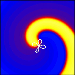
A spiral wave meandering in a sheet of cardiac tissue.

Above is a picture of a meandering spiral wave. Color indicates the transmembrane potential: purple is resting tissue and yellow is depolarized. The thin red band indicates where the transmembrane potential is half way between rest and depolarized. The red region, however, can be in one of two states. The outer red band (next to the deeper purple) is where the transmembrane potential is increasing (depolarizing) during the action potential upstroke, and the inner red band (next to the royal blue) is where the transmembrane potential is decreasing (repolarizing) during the refractory period. The point where the two red bands meet near the center of the tissue is called the phase singularity. There, you can’t tell if the transmembrane potential is increasing or decreasing (to learn more about phase singularities, try Homework Problem 44 in Chapter 10 of IPMB). The spiral wave rotates about the phase singularity, in this case counterclockwise.

One interesting feature about a rotating spiral wave is that its phase singularity sometimes moves around: it meanders. In the above picture, the meander path is white. Often this path looks like it was drawn while playing Spirograph. The motion consists of two parts, each with its own frequency: one corresponds to the rotation of the spiral wave and another creates the petals of the flower-like meander. All this was known long before I entered the field (see, for instance, Art Winfree’s lovely paper: “Varieties of spiral wave behavior: An experimentalist's approach to the theory of excitable media,” Chaos, Volume 1, Pages 303–334, 1991).

What I found in my 1998 paper was that the bidomain nature of cardiac tissue can entrain the two frequencies (force them to be the same, or lock them in to some simple integer ratio). In the bidomain model the intracellular and extracellular spaces are both anisotropic (the electrical resistance depends on direction), but the amount of anisotropy is different in the two spaces. The intracellular space is highly anisotropic and the extracellular space is less so. This property of unequal anisotropy ratios causes the two frequencies to adjust so that the meander path has four-fold symmetry.

My 2004 paper “Art Winfree and the Bidomain Model of Cardiac Tissue” tells the rest of the story (I quote from my original submission, available on ResearchGate, and not the inferior version ultimately published in the Journal of Theoretical Biology).

Most of the mail I get each day is junk, but occasionally, something arrives that has a major impact on my research. One day in June, 2001, I opened my mail to find a letter and preprint from a Canadian mathematician I had never heard of, named Victor LeBlanc. To my astonishment, Victor’s preprint contained analytical proofs specifying what conditions result in locking of the meander pattern to the underlying symmetry of the tissue, and what conditions lead to drift [another type of spiral wave meander]. These conclusions, which I had painstakingly deduced after countless hours of computer simulations, he could prove with paper and pencil. Plus, his analysis predicted many other cases of locking and drifting that I had not examined. I am not enough of a mathematician to understand the proofs, but I could appreciate the results well enough. I contacted Victor, and we tested his predictions using my computer program. The analytical and computational results were consistent in every case we tested. Ironically, Victor predicted that the meander path should have a two-fold symmetry, not the four-fold symmetry that originally motivated my study, and he was correct.... My last email correspondence with Art [Winfree], just a few months before he died, was about a joint paper Victor and I published, describing these results.

I will close with a photo that appeared in the 1997 Annual Report of the Whitaker Foundation, which funded my work on spiral wave meandering. Enjoy!

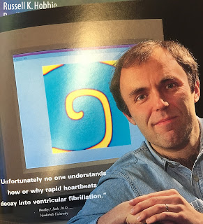
A picture of a spiral wave and me from the 1997 Whitaker Foundation Annual Report.

Cover of the 1997 Whitaker Foundation Annual Report.

Search Engine Optimization and Intermediate Physics for Medicine and Biology

Lately I’ve become fascinated by search engine optimization. My goal is to increase the visibility—and more specifically, the number of pageviews—of this blog. The gurus claim my pagerank will increase if I focus on well-chosen keywords or keyword phrases, so I selected the phrase Intermediate Physics for Medicine and Biology. I’m supposed to use my keyword phrase, Intermediate Physics for Medicine and Biology, often in each post, especially in the first paragraph. I’ve gotten into the habit of using the acronym IPMB for Intermediate Physics for Medicine and Biology, but now I realize this is killing my ranking! I'm a fan of good writing, and this repetition of Intermediate Physics for Medicine and Biology is annoying. So, dear readers, I will avoid repeating the phrase Intermediate Physics for Medicine and Biology too often.

Google helps you refine your selection of keywords. I typed Intermediate Physics for Medicine and Biology into the search bar and looked at the bottom of the page to see popular alternative keyword suggestions.

Popular alternative keywords related to the phrase Intermediate Physics for Medicine and Biology.

Oh my; people are being naughty. I don’t condone illegal downloading, but it’s nice to know somebody wants to read Intermediate Physics for Medicine and Biology.

Many searches are looking for Intermediate Physics for Medicine and Biology's solution manual. Russ Hobbie and I provide the solution manual only to instructors, and we try to keep it off the internet. I hope we have succeeded, but I’m not sure. It’s like trying to stop the tide from coming in. Instructors should forget about Google and just send Russ or me an email. We may require you to jump through hoops to prove you aren’t an imposter, but ultimately we’ll send you the solution manual.

What other strategies have I adopted for search engine optimization? I’ve started using the “description” box in the Blogger software (thank you Mr. Google for letting me use this wonderful software for free!). I’m using “alt text” for images, which helps readers interpret an image if they can’t see it (my real reason for using “alt text,” however, is to up my ranking). They say to compose identifying anchor text for your links, instead of writing “click here.” I now give descriptive names to picture files rather than calling them “picture1.jpg.” I also heard that putting your keyword phrase in bold, italics, and underlining helps: Intermediate Physics for Medicine and Biology. I even read that you should use your keyword phrase as a heading.

Intermediate Physics for Medicine and Biology

Search engines value hyperlinks, so I’m trying to increase the number of links to hobbieroth.blogspot.com. External links are best, but I can’t control them. I can control internal links from one blog post to another, which led to my April 13 creation of the Blog to IPMB Mapping, a shameless orgy of internal linking.

Blogger’s analytics software lets me monitor pageviews. I’ve become addicted to checking these statistics. A few weeks ago a burst of views originated from inside Russia. Someone there read almost every post in one night, binging on Intermediate Physics for Medicine and Biology. My most viewed post is an article about Frank Netter, Medical Illustrator. I don’t know why it’s so popular, but I suspect Google ranking has something to do with it.

Experts recommend repeating your keyword phrase near the end of the post, so I’ll leave you with these final words: Intermediate Physics for Medicine and Biology.

The Radium Girls

The Radium Girls:
The Dark Story of
America's Shining Women,
by Kate Moore.

I recently finished Kate Moore's The Radium Girls: The Dark Story of America’s Shining Women. I chose to read this book because of its relation to topics about radiation risk in Intermediate Physics for Medicine and Biology, but I soon discovered that it isn’t about medical physics. Rather, it focuses on the young women who suffered from occupational radiation exposure. After reviewing previous books about the radium girls, Moore writes:

As a storyteller and a non-academic, I was struck by the fact that the books focused on the legal and scientific aspects of the women’s story, and not on the compelling lives of the girls themselves. In fact, I soon discovered that no book existed that put the radium girls center stage and told the story from their perspective. The individual women who had fought and died for justice had been eclipsed by their historic achievements; they were now known only by the anonymous moniker of “the Radium Girls.” Their unique experiences—their losses and their loves; their triumphs and their terrors—had been forgotten, if ever charted in the first place.

I became determined to correct that omission.

The job of a radium girl was to paint luminous dials on clocks and instruments, so you could see them in the dark. They used a radioluminescent paint containing radioactive radium mixed with a scintillator such as zinc-sulfide. Most worked for either the United States Radium Corporation in Orange, New Jersey, or the Radium Dial Company in Ottawa, Illinois. Their supervisors taught them to make a fine point on their paint brush by putting it in their mouth, a process called lip-pointing. Each time they lip-pointed, they ingested a bit of radium.

Radium girls lip-pointing in a dial factory: “Lip, Dip, Paint.” From Wikipedia.

Moore examines the individual lives of these girls—many in their 20s, some in their teens—and explains their physical symptoms and health problems in excruciating detail. Don’t read the book if you’re squeamish; for instance, one of the first symptoms was a tooth ache, but when a dentist extracted the tooth a chunk of the jaw would come out too. Radium—an alpha emitter in the same column of the periodic table as calcium—is taken up by bones. With a half-life of 1600 years, it irradiates the bones throughout the girl’s life.

The heroes of this story are women like Grace Fryer and Catherine Donohue, who demanded justice for themselves and other victims. The villains are the leaders of the corporations. I had some sympathy for these companies at first, because the dangers from radiation were not well understood in the 1920s, so how could they know? But as time went by and the hazards became obvious, the executives denied the facts and covered up the risks. By the book’s end, these men personify evil.

Sometimes I get frustrated when people believe conspiracy theories and fairy tales about the danger from low levels of radiation, but The Radium Girls helps me understand why it happens. When people in authority ignore the risk to others for their own profit and then lie about it, they undermine trust, until no one believes even the most solid science.

If you are driving through Illinois on I-80, stop in Ottawa and see the statue of a dial painter. Moore describes its creation:

For a long time—too long—the legacy of the radium girls was recorded only in the law books and in scientific files. But in 2006, an eighth-grade Illinois student called Madeline Piller read a book on the dial-painters by Dr. Ross Mullner. “No monuments,” he wrote, “have ever been erected in their memory.”

Madeline was determined to change that. “They deserve to be remembered,” she said. “Their courage brought forth federal health standards. I want people to know [there] is a memorial to these brave women.”

When she began to champion her cause, she found that Ottawa, at last, was ready to honor its native heroines and their comrades-in-arms. The town held fish-fry fund-raisers and staged plays to secure the $80,000 needed. “The mayor was supportive,” said Len Grossman. “It was a complete turnaround. That was wonderful to see.”

On September 2, 2011, the bronze statue for the dial-painters was unveiled by the governor in Ottawa, Illinois. It is a statue of a young woman from the 1920’s, with a paintbrush in one hand and a tulip in the other, standing on a clock face. Her skirt swishes, as though at any moment she might step down from her time-ticking pedestal and come to life.

The blog Backyard Tourist has excellent photos of the statue.

The Radium Girls doesn’t explain much of the physics behind radiation exposure, but it does remind us why we study medical physics. For a history lesson, a case study in occupational safety, an inspirational story, and a great read, I recommend The Radium Girls.

The Radium Girls discusses radiation risk, a topic covered in Section 16.12 of
Intermediate Physics for Medicine and Biology.

A YouTube video of Kate Moore talking about her book The Radium Girls.

Sepulveda, Roth and Wikswo (1989): How to Write a Scientific Paper

In 1989, Nestor Sepulveda, John Wikswo and I published “Current Injection into a Two-Dimensional Anisotropic Bidomain” (Biophysical Journal, 55:987–999). Of my papers, this is one of my favorites.

When I teach my graduate Bioelectric Phenomena class here at Oakland University, we study the Sepulveda et al. (1989) article. The primary goal of the class is to introduce students to bioelectricity, but a secondary goal is to analyze how to write scientific papers. When we get to our paper, I let students learn the scientific content from the publication itself. Instead, I use class time to analyze scientific writing. The paper lends itself to this task: It is written well enough to serve as an example of technical writing, but it is written poorly enough to illustrate how writing can be improved. Critically tearing apart the writing of someone else’s paper in front of students would be rude, but because this writing is partly mine I don’t feel guilty.

Many readers of Intermediate Physics for Medicine and Biology will eventually write papers of their own, so in this post I share my analysis of scientific writing just as I present it in class. Students read “Current Injection into a Two-Dimensional Anisotropic Bidomain” in advance, and then during class we go through the writing page by page, and often line by line, using a powerpoint presentation that I have placed on the IPMB website. I use the “animation” feature of powerpoint so edits, revisions, and corrections can be considered one at a time. To see for yourself, download the powerpoint and click “slide show.” Then, start using the right arrow to analyze the paper.

A screen shot of the first page of the powerpoint. It looks a mess, but the animation feature lets you consider all these suggestions one by one. You can download it and use it to teach your students.

When using this powerpoint, keep these points in mind:

• One reason I use Sepulveda et al. (1989) as my example is that it has the classic format of a scientific paper: Introduction, Methods, Results, and Discussion. It also contains an Abstract, References, and other sections of a scientific publication. 
• Often I highlight a sentence or two of text and ask students to revise and improve it. If you are leading a class using this powerpoint, stop and let the students struggle with the revision. Then compare their revised text with mine. The class should be interactive.
• I have talked before in this blog about the importance of writing. In the powerpoint, I mention two publications that have helped me become a better writer. First is Strunk and White’s book Elements of Style. The powerpoint illustrates much of their advice—such as their famous admonition to “omit needless words”—with concrete examples. You can read Elements of Style online here. Second is N. David Mermin’s essay “What’s Wrong with These Equations” published in Physics Today (download it here). Mermin explains how to integrate math with prose, and introduces the “Good Samaritan Rule” (remind your reader what an equation is about when you refer to it, rather than just saying “Eq. 4”) and other concepts. 
• Some of the points raised in my powerpoint are trivial, such as the difference between “there,” “their,” and “they’re.” Others are more substantial, such as sentence construction and clarity. I find it takes most of a 90 minute class to finish the whole thing. 
• On the sixth page of the powerpoint I have a note reminding me to “Tell Story.” The story is one I wrote about in the original version of my paper “Art Winfree and the Bidomain Model of Cardiac Tissue.” “Nestor Sepulveda, a research assistant professor from Columbia who was working in John [Wikswo]'s lab, had written a finite element computer program that we modified to do bidomain calculations. One of the first simulations he performed was of the transmembrane potential induced in a two-dimensional sheet of cardiac tissue having 'unequal anisotropy ratios' (different degrees of anisotropy in the intracellular and extracellular spaces). Much to our surprise, Nestor found that when he stimulated the tissue through a small cathodal electrode, depolarization (a positive transmembrane potential) appeared under the electrode, but hyperpolarization (a negative transmembrane potential) appeared near the electrode along the fiber direction (Fig. 2). The depolarization was stronger in the direction perpendicular to the fibers, giving those voltage contour lines a shape that John named the ‘dogbone.’ Only Nestor understood the details of his finite element code, and I was a bit worried that his program might contain a bug that caused this weird result. So I quietly returned to my office and developed an entirely different numerical scheme, using Fourier transforms, to do the same calculation. Of course, I got the same result Nestor did (there was no bug). Although I didn’t realize it then, I would spend the next 15 years exploring the implications of Nestor’s result.” During class, I often take off on tangents telling old  “war stories” like this. I can’t help myself.
• John Wikswo, my coauthor and PhD dissertation advisor, is still active, and he and I continue to collaborate. I learned much about scientific writing from him, but our writing styles are different and he might not agree with all the suggestions in the powerpoint. Tragically, Nestor Sepulveda has passed away; a great loss for bioelectricity research. I miss him.
• If you are teaching and want to discuss how to write a scientific paper, feel free to use this powerpoint. I encourage you to download it and modify it to suit your needs. Students could even use it for self study, although they would not see some essential hand waving.

Although the powerpoint suggests many changes to the Sepulveda et al. (1989) paper, I nevertheless consider that article to be a success. According to Google Scholar, it has been cited 379 times. I believe it had an impact on the field of pacing and defibrillation of the heart. Overall, I am proud of the writing.

Let me close by emphasizing that writing is an art. Your style might not be the same as mine. Take my suggestions in the powerpoint as just that: suggestions. Yet, whether or not you agree with my suggestions, I believe your students will benefit by going through the process of revising a scientific paper. It’s the next best thing to assigning them to write their own paper. Enjoy!

The Constituents of Blood

I’m a big supporter of blood donation. This week I gave another pint to the Red Cross, which brings my total to 8 gallons. As I lay there with a needle stuck in my arm, I began to wonder “what’s in this blood they’re squeezing out of me?”

Table 3.1 in Intermediate Physics for Medicine and Biology lists some constituents of blood. I reproduce the table below, with revisions.

Constituent	Density in mg/cm3	Number in 1 μm3
Water	1000	33,000,000,000
Sodium	3	83,000,000
Glucose	1	3,300,000
Cholesterol	2	3,100,000
Hemoglobin	150	1,400,000
Albumin	45	390,000

This version of the table highlights several points. Water molecules outnumber all others by a factor of four hundred. Sodium ions are sixty times more common than hemoglobin molecules, but the mass density of hemoglobin is over fifty times that of sodium. In other words, if judged by number of molecules (and therefore the osmotic effect) sodium is most important, but if judged by mass or volume fraction, hemoglobin dominates. Glucose and cholesterol are intermediate cases. Albumin has a surprisingly small number of molecules, given that I thought it was one of the main contributors to osmotic pressure. It is a big molecule, however, so by mass it contributes nearly a third as much as hemoglobin.

Are other molecules in blood important? You can find a comprehensive list of blood constituents beautifully illustrated here. When judged by number, sodium is the most important small ion, but the chloride ion contributes nearly as much. Carbon dioxide and bicarbonate are also significant, and potassium has about the same number of molecules as glucose. If you drive drunk, you may have twice as many ethyl alcohol molecules as potassium ions (if the number of ethanol molecules reaches the level of sodium or chloride ions, you die). Urea has a similar number of molecules as hemoglobin.

Judged by mass, you get an entirely different picture. Large protein molecules dominate. Hemoglobin is by far the largest contributor to blood by mass (after water, of course), followed by albumin and another group of proteins called globulins. Next are glycoproteins such as the clotting factor fibrinogen and iron-binding transferrin.

Many trace constituents hardly affect the osmotic pressure or density of blood, but are excellent biomarkers for diagnosing diseases.

If you’re starting to think that blood is awfully crowded, you’re right. The picture below is by David Goodsell. No scale bar is included, but each candy-apple-red hemoglobin molecule in the lower left has a diameter of about 6 nm. The water, ions, and other small molecules such as glucose are not shown; if they had been they would produce a fine granular appearance (water has diameter of about 0.3 nm) filling in the spaces between the larger macromolecules.

Blood. Serum is in the upper right and a red blood cell is in the lower left. In the serum, the Y-shaped molecules are antibodies (an immunoglobulin), the long thin light-red molecules are fibrinogen (a glycoprotein), and the numerous potato-like yellow proteins are albumin. The red blood cell is filled with red hemoglobin molecules. The cell membrane is in purple. The illustration is by David S. Goodsell of the Scripps Research Institute.

In another eight weeks I will get free juice and cookies be eligible to give blood again. It doesn’t hurt (much) or take (too) long. If you want to donate, contact the American Red Cross. Give the gift of life.

A Biological Constant

Membranes, Ions
and Impulses,
by Kenneth Cole

Physics has many famous constants: Planck’s constant, the speed of light, and the gravitational constant, to name a few. Biology has few such constants. Life is so full of variety that almost any parameter can vary between species or tissues. In fact, physicists differ from biologists by their focus on the unity rather than the diversity of life.

There is, however, one parameter that comes close to being a biological constant. All cells are surrounded by a membrane whose thickness and composition varies little among species. Therefore, the capacitance per unit area, C_m, of a membrane is as close to being a biological constant as you are likely to find.

In Section 6.17 of Intermediate Physics for Medicine and Biology, Russ Hobbie and I calculate the capacitance of a lipid bilayer, and find that C_m is about 0.01 farads per square meter. Many of the key papers during the “golden age” of classical biophysics didn’t use standard SI units. Instead of measuring distance in meters, they used centimeters. If you express C_m as per square centimeter, and if you use microfarads instead of farads, you get the easy-to-remember value of C_m = 1 μF/cm². Kenneth Cole wrote in his book Membranes, Ions and Impulses: A Chapter of Classical Biophysics

This figure of about 1 μF/cm² has been so confirmed and refined, extended and approximated for membranes of red cells and almost all other living cells, as to become a biophysical constant.

Are there other biological constants? I suppose some constants governing the structure of key biological molecules, such as the distance between adjacent base pairs of the DNA double helix (0.34 nm), are conserved throughout biology. But these parameters belong more to the realm of biochemistry than biophysics. If you restrict your selection to parameters discussed in IPMB, C_m is one of the few biological constants.

Membranes, Ions and Impulses, by Kenneth Cole.

 

 

The Curie Temperature

In Chapter 8 of Intermediate Physics for Medicine and Biology, Russ Hobbie and I discuss magnetic materials, including ferromagnets (permanent magnets in which electron spins are aligned even in the absence of an external magnetic field). We write

If the temperature of the sample is raised above a critical temperature called the Curie temperature, the magnetism is destroyed.

When seeing such a sentence, my first inclination is to write a homework problem that uses a toy model to illustrate the physics behind the concept. Unfortunately, analyzing the Curie temperature is difficult, so no new homework problem appears in this post (readers are encouraged to try their hand at writing one).

Solid State Physics,
by Ashcroft and Mermin.

When faced with a difficult concept in material physics, I reach for a copy of Solid State Physics by Neil Ashcroft and N. David Mermin. Regular readers of this blog may recall that I am a big fan of Mermin (for instance, see here and here). Everything I know about solid state physics (which isn’t much) I learned from Solid State Physics. When Ashcroft and Mermin describe magnetic ordering of spins, they explain that

Quantitative theories of magnetic ordering have proved most difficult to construct near the critical temperature T_c at which ordering disappears. The difficulty is not peculiar to the problem of magnetism. The critical points of liquid-vapor transitions, superconducting transitions (Chapter 34), the superfluid transition in liquid He₄, and order-disorder transitions in alloys, to name just a few, present quite strong analogies and give rise to quite similar theoretical difficulties.

They settle for a phenomenological description of the Curie temperature.

The critical temperature T_c above which magnetic ordering vanishes is known as the Curie temperature in ferromagnets… As the critical temperature is approached from below, the spontaneous magnetization…drops continuously to zero. The observed magnetization just below T_c is well described by a power law.

M(T) ∼ (T_c – T)^β,

where β is typically between 0.33 and 0.37.

Below I plot of the spontaneous magnetization M versus the absolute temperature T for β=1/3.

The Curie temperature is interesting for two reasons. First, it is not named after Marie Curie, who plays such a big role in medical physics for isolating some of the first radioactive elements including radium and polonium. Instead, it is named after her husband Pierre Curie, who did important research on magnetism. Second, the ferromagnetic material that Russ and I discuss most in IPMB is magnetite (Fe₃O₄), which is found in magnetosomes, small magnetic particles that cause magnetotactic bacteria to align with the earth's magnetic field. The Curie temperature for magnetite is 585 °C, or 858 K, which is too hot to support life. Perhaps other substances exist for which the Curie temperature plays a role in biology and medicine, but I don’t know what they are.

I conclude with a quote from Mermin’s delightful essay “Writing Physics” in which he talks about writing Solid State Physics with Ashcroft. Enjoy!

The striking exception to my inability to write collaboratively is my eight-year collaboration with Neil Ashcroft on our 800 page book on solid state physics. We have very different prose styles. Yet the book has a clear and distinctive uniform tone, which can't be identified as belonging to either of us. I think the reason this worked was that Neil knows solid state physics much better than I do. So he would produce the first drafts. Characteristically, I would not understand them. So I would try to make sense of what he was saying, and then produce my typical kind of irritating second draft. Neil, however, would now have to correct all my mistakes in a massively rewritten third draft. I would then have to root out any new obscurities he had introduced in a fourth draft. By this kind of tennis-playing, we would go through five or six drafts, and emerge with something that was clear, correct, and sounded like a human voice. That voice, however, was neither of ours.