In my more contemplative moments, I sometimes ponder: who am I? Or perhaps better: what am I? In my personal life I am many things: son, husband, father, brother, dog-lover, die-hard Cubs fan, Asimov aficionado, Dickens devotee, and mid-twentieth-century-Broadway-musical-theatre admirer.
What I am professionally is not as clear. By training I’m a physicist. Each month I read Physics Today and my favorite publication is the American Journal of Physics. But in many ways I don’t fit well in physics. I don’t understand much of what’s said at our weekly physics colloquium, and I have little or no interest in topics such as high energy physics. Quantum mechanics frightens me.
The term biophysicist doesn’t apply to me, because I don’t work at the microscopic level. I don’t care about protein structures or DNA replication mechanisms. I’m a macroscopic guy.
My work overlaps that of biomedical engineers, and indeed I publish frequently in biomedical engineering journals. But my work is not applied enough for engineering. In the 1990s, when searching desperately for a job, I considered positions in biomedical engineering departments, but I was never sure what I would teach. I have no idea what’s taught in engineering schools. Ultimately I decided that I fit better in a physics department.
Mathematical biologist is a better definition of me. I build mathematical models of biological systems for a living. But I’m at heart neither a mathematician nor a biologist. I find math papers—full of theorem-proof-theorem-proof—to be tedious. Biologists celebrate life’s diversity, which is exactly the part of biology I like to sweep under the rug.
I’m not a medical physicist. Nothing I have worked on has healed anyone. Besides, medical physicists work in nuclear medicine and radiation therapy departments at hospitals, and they get paid a lot more that I do. No, I’m definitely not a medical physicist. Perhaps one of the most appropriate labels is biological physicist—whatever that means.
Another question is: at what level do I work? I’m not a popularizer of science or a science writer (except when writing this blog, which is more of a hobby; my “Hobbie hobby”). I write research papers and publish them in professional journals. Yet, in these papers I build toy models that are as simple as possible (but no simpler!). Reviewers of my manuscripts write things like “the topic is interesting and the paper is well-written, but the model is too simple; it fails to capture the underlying complexity of the system.” When my simple models grow too complicated, I change direction and work on something else. So my research is neither at an introductory level nor an advanced level.
I guess the best label for me is: Intermediate Physicist for Medicine and Biology.
Friday, November 25, 2016
Friday, November 18, 2016
Molybdenum-99 for Medical Imaging
| Molybdenum-99 for Medical Imaging, published by the National Academies Press. |
Recently, the Committee on State of Molybdenum-99 Production and Utilization and Progress Toward Eliminating Use of Highly Enriched Uranium addressed this issue in their report Molybdenum-99 for Medical Imaging, published by the National Academies Press. Below I reproduce excerpts from the executive summary.
This Academies study was mandated by the American Medical Isotopes Production Act of 2012. Key results for each of the five study charges are summarized below…News articles associated with the release of the report can be found here, here, here, and here. The message I get from this report is that the long-term prognosis for 99Mo supplies is promising, but the short-term outlook is worrisome. Let us hope I’m too pessimistic.
Study charge 1: Provide a list of facilities that produce molybdenum-99 (Mo-99) for medical use including an indication of whether these facilities utilize highly enriched uranium (HEU)… About 95 percent of the global supply of Mo-99 for medical use is produced in seven research reactors and supplied from five target processing facilities located in Australia, Canada, Europe, and South Africa. About 5 percent of the global supply is produced in other locations for regional use. About 75 percent of the global supply of Mo-99 for medical use is produced using HEU targets; the remaining 25 percent is produced with low enriched uranium targets….
Study charge 2: Review international production of Mo-99 over the previous 5 years … New Mo-99 suppliers have entered the global supply market since 2009 and further expansions are planned. An organization in Australia (Australian Nuclear Science and Technology Organisation) has become a global supplier and is currently expanding its available supply capacity; existing global suppliers in Europe (Mallinckrodt) and South Africa (NTP Radioisotopes) are also expanding ... A reactor in France (OSIRIS) that produced Mo-99 shut down permanently in December 2015. The reactor in Canada (NRU) will stop the routine production of Mo-99 after October 2016 and permanently shut down at the end of March 2018.
Study charge 3: Assess progress made in the previous 5 years toward establishing domestic production of Mo-99 and associated medical isotopes iodine-131 (I-131) and xenon-133 (Xe-133) … The American Medical Isotopes Production Act of 2012 and financial support from the Department of Energy’s National Nuclear Security Administration … have stimulated private-sector efforts to establish domestic production of Mo-99 and associated medical isotopes. Four NNSA-supported projects and several other private-sector efforts are under way to establish domestic capabilities to produce Mo-99; each project is intended to supply half or more of U.S. needs…. it is unlikely that substantial domestic supplies of Mo-99 will be available before 2018. Neither I-131 nor Xe-133 is currently produced in the United States, but one U.S. organization (University of Missouri Research Reactor Center) is developing the capability to supply I-131; some potential domestic Mo-99 suppliers also have plans to supply I-131 and/or Xe-133 in the future.
Study charge 4: Assess the adequacy of Mo-99 supplies to meet future domestic medical needs, particularly in 2016 and beyond …The United States currently consumes about half of the global supply of Mo-99/technetium-99m (Tc-99m) for medical use; global supplies of Mo-99 are adequate at present to meet domestic needs. Domestic demand for Mo-99/Tc-99m has been declining for at least a decade and has declined by about 25 percent between 2009-2010 and 2014-2015; domestic medical use of Mo-99/Tc-99m is unlikely to increase significantly over the next 5 years. The committee judges that there is a substantial ... likelihood of severe Mo-99/Tc-99m supply shortages after October 2016, when Canada stops supplying Mo-99, lasting at least until current global Mo-99 suppliers complete their planned capacity expansions (planned for 2017) and substantial new domestic Mo-99 supplies enter the market (not likely until 2018 and beyond)….
Study charge 5: Assess progress made by the DOE and others to eliminate worldwide use of HEU in reactor targets and medical isotope production facilities and identify key remaining obstacles for eliminating HEU use… The American Medical Isotopes Production Act of 2012 is accelerating the elimination of worldwide use of HEU for medical isotope production [to reduce the amount of HEU available for production of weapons of mass destruction by terrorist groups]. Current global Mo-99 suppliers have committed to eliminating HEU use in reactor targets and medical isotope production facilities and are making uneven progress toward this goal. Progress is … being impeded by the continued availability of Mo-99 produced with HEU targets … Even after HEU is eliminated from Mo-99 production, large quantities of HEU-bearing wastes from past production will continue to exist at multiple locations throughout the world…
Friday, November 11, 2016
Mathematical Physiology
 |
| Mathematical Physiology, by James Keener and James Sneyd. |
It can be argued that of all the biological sciences, physiology is the one in which mathematics has played the greatest role. From the work of Helmholtz and Frank in the last century through to that of Hodgkin, Huxley, and many others in this century [the first edition of MP was published in 1998], physiologists have repeatedly used mathematical methods and models to help their understanding of physiological processes. It might thus be expected that a close connection between applied mathematics and physiology would have developed naturally, but unfortunately, until recently, such has not been the case.If you substitute the words “physics” for “mathematics,” “physical” for “mathematical,” and “physicist” for “mathematician,” you would almost think that this preface had been written by Russ Hobbie for an early edition of IPMB.
There are always barriers to communication between disciplines. Despite the quantitative nature of their subject, many physiologists seek only verbal descriptions, naming and learning the functions of an incredibly complicated array of components; often the complexity of the problem appears to preclude a mathematical description. Others want to become physicians, and so have little time for mathematics other than to learn about drug dosages, office accounting practices, and malpractice liability. Still others choose to study physiology precisely because thereby they hope not to study more mathematics, and that in itself is a significant benefit. On the other hand, many applied mathematicians are concerned with theoretical results, proving theorems and such, and prefer not to pay attention to real data or the applications of their results. Others hesitate to jump into a new discipline, with all its required background reading and its own history of modeling that must be learned.
But times are changing, and it is rapidly becoming apparent that applied mathematics and physiology have a great deal to offer one another. It is our view that teaching physiology without a mathematical description of the underlying dynamical processes is like teaching planetary motion to physicists without mentioning or using Kepler’s laws; you can observe that there is a full moon every 28 days, but without Kepler’s laws you cannot determine when the next total lunar or solar eclipse will be nor when Halley’s comet will return. Your head will be full of interesting and important facts, but it is difficult to organize those facts unless they are given a quantitative description. Similarly, if applied mathematicians were to ignore physiology, they would be losing the opportunity to study an extremely rich and interesting field of science.
To explain the goals of this book, it is most convenient to begin by emphasizing what this book is not; it is not a physiology book, and neither is it a mathematics book. Any reader who is seriously interested in learning physiology would be well advised to consult an introductory physiology book such as Guyton and Hall (1996) or Berne and Levy (1993), as, indeed, we ourselves have done many times. We give only a brief background for each physiological problem we discuss, certainly not enough to satisfy a real physiologist. Neither is this a book for learning mathematics. Of course, a great deal of mathematics is used throughout, but any reader who is not already familiar with the basic techniques would again be well advised to learn the material elsewhere.
Instead, this book describes work that lies on the border between mathematics and physiology; it describes ways in which mathematics may be used to give insight into physiological questions, and how physiological questions can, in turn, lead to new mathematical problems. In this sense, it is truly an interdisciplinary text, which, we hope, will be appreciated by physiologists interested in theoretical approaches to their subject as well as by mathematicians interested in learning new areas of application.
Many of the topics in MP overlap those in IPMB: diffusion, bioelectricity, osmosis, ion channels, blood flow, and the heart. MP covers additional topics not in IPMB, such as biochemical reactions, calcium dynamics, bursting pancreatic beta cells, and the regulation of gene expression. What IPMB has that MP doesn’t is clinical medical physics: ultrasound, x-rays, tomography, nuclear medicine, and MRI. Both books assume a knowledge of calculus, both average many equations per page, and both have generous collections of homework problems.
Which book should you use? Mathematical Physiology won an award, but Intermediate Physics for Medicine and Biology has an award-winning blog. I’ll take the book with the blog. I bet I know what Frankie will say: “I’ll take both!”
Friday, November 4, 2016
I Spy Physiology
Last year I wrote a blog post about learning biology, aimed at physicists who wanted an introduction to biological ideas. Today, let’s suppose you have completed your introduction to biology. What’s next? Physiology!
What is physiology? Here is the answer provided by the website physiologyinfo.org, sponsored by the American Physiological Society.
My favorite part of physiologyinfo.org is the I Spy Physiology blog.
My only complaint about physiologyinfo.org is its lack of physics. That is where Intermediate Physics for Medicine and Biology comes in: IPMB puts the physics in the physiology.
What is physiology? Here is the answer provided by the website physiologyinfo.org, sponsored by the American Physiological Society.
Physiology is the study of how the human body works under normal conditions. You use physiology when you exercise, read, breathe, eat, sleep, move or do just about anything.
Physiology is generally divided into ten physiological organ systems: the cardiovascular system, the respiratory system, the immune system, the endocrine system, the digestive system, the nervous system, the renal system, the muscular system, the skeletal system, and the reproductive system.
 |
| Screenshot of the I Spy Physiology website. |
At the American Physiological Society (APS), we believe that physiology is everywhere. It is the foundational science that provides the backbone to our understanding of health and medicine. At its core, physiology is all about understanding the healthy (normal) state of animals—humans included!—what happens when something goes wrong (the abnormal state) and how to get things back to working order. Physiologists study these normal and abnormal states at all levels of the organism: from tiny settings like in a cell to large ones like the whole animal. We also study how humans and animals function, including how they eat, breathe, survive, exercise, heal and sense the environment around them.Other parts of the website I like are “Quizzes and Polls” (I aced the cardiovascular system quiz!) and the podcast library. As a Michigander, I was pleased to see the article about William Beaumont. Finally, I enjoyed Dr. Dolittle’s delightful blog Life Lines, about comparative physiology.
On this blog, we’ll endeavor to answer the questions “What is physiology?”, “Where is physiology?”, and “Why does it matter to you?” through current news and health articles and research snippets highlighted by APS members and staff. We’ll also explore the multifaceted world of physiology and follow the path from the lab all the way to the healthy lifestyle recommendations that you receive from your doctor
My only complaint about physiologyinfo.org is its lack of physics. That is where Intermediate Physics for Medicine and Biology comes in: IPMB puts the physics in the physiology.
Friday, October 28, 2016
dGEMRIC
dGEMRIC is an acronym for delayed gadolinium enhanced magnetic resonance imaging of cartilage. Adil Bashir and his colleagues provide a clear introduction to dGEMRIC in the abstract of their paper “Nondestructive Imaging of Human Cartilage Glycosaminoglycan Concentration by MRI”
(Magnetic Resonance in Medicine, Volume 41, Pages 857–865, 1999).
The method is based on Donnan equilibrium, which Russ Hobbie and I describe in Section 9.1 of Intermediate Physics for Medicine and Biology. Assume the cartilage tissue (t) is bathed by saline (b). We will ignore all ions except the sodium cation, the chloride anion, and the negatively charged glycosaminoglycan (GAG). Cartilage is not enclosed by a semipermeable membrane, as analyzed in IPMB. Instead, the GAG molecules are fixed and immobile, so they act as if they cannot cross a membrane surrounding the tissue. Both the tissue and bath are electrically neutral, so [Na+]b = [Cl-]b and [Na+]t = [Cl-]t + [GAG-], where we assume GAG is singly charged (we could instead just interpret [GAG-] as being the fixed charge density). At the cartilage surface, sodium and chloride are distributed by a Boltzmann factor: [Na+]t/[Na+]b = [Cl-]b/[Cl-]t = exp(-eV/kT), where V is the electrical potential of the tissue relative to the bath, e is the elementary charge, k is the Boltzmann constant, and T is the absolute temperature. We can solve these equations for [GAG-] in terms of the sodium concentrations: [GAG-] = [Na+]b ( [Na+]t/[Na+]b - [Na+]b/[Na+]t ).
Now, suppose you add a small amount of gadolinium diethylene triamine pentaacetic acid (Gd-DTPA2-); so little that you can ignore it in the equations of neutrality above. The concentrations of Gd-DTPA on the two sides of the articular surface are related by the Boltzmann factor [Gd-DTPA2-]b/[Gd-DTPA2-]t = exp(-2eV/kT) [note the factor of two in the exponent reflecting the valance -2 of Gd-DTPA], implying that [Gd-DTPA2-]b/[Gd-DTPA2-]t = ( [Na+]t/[Na+]b )2. Therefore,

We can determine [GAG-] by measuring the sodium concentration in the bath and the Gd-DTPA concentration in the bath and the tissue. Section 18.6 of IPMB describes how gadolinium shortens the T1 time constant of a magnetic resonance signal, so using T1-weighted magnetic resonance imaging you can determine the gadolinium concentration in both the bath and the tissue.
From my perspective, I like dGEMRIC because it takes two seemingly disparate parts of IPMB, the section of Donnan equilibrium and the section on how relaxation times affect magnetic resonance imaging, and combines them to create an innovative imaging method. Bashir et al.’s paper is eloquent, so I will close this blog post with their own words.
Despite the compelling need mandated by the prevalence and morbidity of degenerative cartilage diseases, it is extremely difficult to study disease progression and therapeutic efficacy, either in vitro or in vivo (clinically). This is partly because no techniques have been available for nondestructively visualizing the distribution of functionally important macromolecules in living cartilage. Here we describe and validate a technique to image the glycosaminoglycan concentration ([GAG]) of human cartilage nondestructively by magnetic resonance imaging (MRI). The technique is based on the premise that the negatively charged contrast agent gadolinium diethylene triamine pentaacetic acid (Gd(DTPA)2-) will distribute in cartilage in inverse relation to the negatively charged GAG concentration. Nuclear magnetic resonance spectroscopy studies of cartilage explants demonstrated that there was an approximately linear relationship between T1 (in the presence of Gd(DTPA)2-) and [GAG] over a large range of [GAG]. Furthermore, there was a strong agreement between the [GAG] calculated from [Gd(DTPA)2-] and the actual [GAG] determined from the validated methods of calculations from [Na+] and the biochemical DMMB assay. Spatial distributions of GAG were easily observed in T1-weighted and T1-calculated MRI studies of intact human joints, with good histological correlation. Furthermore, in vivo clinical images of T1 in the presence of Gd(DTPA)2- (i.e., GAG distribution) correlated well with the validated ex vivo results after total knee replacement surgery, showing that it is feasible to monitor GAG distribution in vivo. This approach gives us the opportunity to image directly the concentration of GAG, a major and critically important macromolecule in human cartilage.
 |
| A schematic illustration of the structure of cartilage. |
Now, suppose you add a small amount of gadolinium diethylene triamine pentaacetic acid (Gd-DTPA2-); so little that you can ignore it in the equations of neutrality above. The concentrations of Gd-DTPA on the two sides of the articular surface are related by the Boltzmann factor [Gd-DTPA2-]b/[Gd-DTPA2-]t = exp(-2eV/kT) [note the factor of two in the exponent reflecting the valance -2 of Gd-DTPA], implying that [Gd-DTPA2-]b/[Gd-DTPA2-]t = ( [Na+]t/[Na+]b )2. Therefore,
We can determine [GAG-] by measuring the sodium concentration in the bath and the Gd-DTPA concentration in the bath and the tissue. Section 18.6 of IPMB describes how gadolinium shortens the T1 time constant of a magnetic resonance signal, so using T1-weighted magnetic resonance imaging you can determine the gadolinium concentration in both the bath and the tissue.
From my perspective, I like dGEMRIC because it takes two seemingly disparate parts of IPMB, the section of Donnan equilibrium and the section on how relaxation times affect magnetic resonance imaging, and combines them to create an innovative imaging method. Bashir et al.’s paper is eloquent, so I will close this blog post with their own words.
The results of this study have demonstrated that human cartilage GAG concentration can be measured and quantified in vitro in normal and degenerated tissue using magnetic resonance spectroscopy in the presence of the ionic contrast agent Gd(DTPA)2- … These spectroscopic studies therefore demonstrate the quantitative correspondence between tissue T1 in the presence of Gd(DTPA)2- and [GAG] in human cartilage. Applying the same principle in an imaging mode to obtain T1 measured on a spatially localized basis (i.e., T1-calculated images), spatial variations in [GAG] were visualized and quantified in excised intact samples…
In summary, the data presented here demonstrate the validity of the method for imaging GAG concentration in human cartilage… We now have a unique opportunity to study developmental and degenerative disease processes in cartilage and monitor the efficacy of medical and surgical therapeutic measures, for ultimately achieving a greater understanding of cartilage physiology in health and disease.
Friday, October 21, 2016
The Nuts and Bolts of Life: Willem Kolff and the Invention of the Kidney Machine
 |
| The Nuts and Bolts of Life: Willem Kolff and the Invention of the Kidney Machine, by Paul Heiney. |
Two compartments, the body fluid and the dialysis fluid, are separated by a membrane that is porous to the small molecules to be removed and impermeable to larger molecules. If such a configuration is maintained long enough, then the concentration of any solute that can pass through the membrane will become the same on both sides.The history of the artificial kidney is fascinating. Paul Heiney describes this story in his book The Nuts and Bolts of Life: Willem Kolff and the Invention of the Kidney Machine.
Willem Kolff…has battled to mend broken bodies by bringing mechanical solutions to medical problems. He built the first ever artificial kidney and a working artificial heart, and helped create the artificial eye. He s the true founder of the bionic age in which all human parts will be replaceable.Heiney’s book is not a scholarly treatise and there is little physics in it, but Kolff’s personal story is captivating. Much of the work to develop the artificial kidney was done during World War II, when Kolff’s homeland, the Netherlands, was occupied by the Nazis. Kolff managed to create the first artificial organ while simultaneously caring for his patients, collaborating with the Dutch resistance, and raising five children. Kolff was a tinkerer in the best sense of the word, and his eccentric personality reminds me of the inventor of the implantable pacemaker, Wilson Greatbatch.
Below are some excepts from the first chapter of The Nuts and Bolts of Life. To learn more about Kolff, see his New York Times obituary.
What might a casual visitor have imagined was happening behind the closed door of Room 12a on the first floor of Kampen Hospital in a remote and rural corner of Holland on the night of 11 September 1945? There was little to suggest a small miracle was taking place; in fact, the sounds that emerged from that room could easily have been mistaken for an organized assault.
The sounds themselves were certainly sinister. There was a rumbling that echoed along the tiled corridors of the small hospital and kept patients on the floor below from their sleep; and the sound of what might be a paddle-steamer thrashing through water. All very curious…
The 67-year-old patient lying in Room 12a would have been oblivious to all this. During the previous week she had suffered high fever, jaundice, inflammation of the gall bladder and kidney failure. Not quite comatose, she could just about respond to shouts or the deliberative infliction of pain. Her skin was pale yellow and the tiny amount of urine she produced was dark brown and cloudy….
Before she was wheeled into Room 12a of Kampen Hospital that night, Sofia Schafstadt’s death was a foregone conclusion. There was no cure for her suffering; her kidneys were failing to cleanse her body of the waste it created in the chemical processes of keeping her alive. She was sinking into a body awash in her own poisons….
But that night was to be like no other night in medical history. The young doctor, Willem Kolff, then aged thirty-four and an internist at Kampen Hospital, brought to a great crescendo his work of much of the previous five years. That night, he connected Sofia Schafstadt to his artificial kidney – a machine born out of his own ingenuity. With it, he believed, for the first time ever he could replicate the function of one of the vital organs with a machine working outside the body…
The machine itself was the size of a sideboard and stood by the patient’s bed. The iron frame carried a large enamel tank containing fluid. Inside this rotated a drum around which was wrapped the unlikely sausage skin through which the patient’s blood flowed. And that, in essence, was it: a machine that could undoubtedly be called a contraption was about to become the world’s first successful artificial kidney…
Friday, October 14, 2016
John David Jackson (1925-2016)
 |
| Classical Electrodynamics, 3rd Ed, by John David Jackson. |
The classical analog of Compton scattering is Thomson scattering of an electromagnetic wave by a free electron. The electron experiences the electric field E of an incident plane electromagnetic wave and therefore has an acceleration −eE/m. Accelerated charges radiate electromagnetic waves, and the energy radiated in different directions can be calculated, giving Eqs. 15.17 and 15.19. (See, for example, Jackson 1999, Chap. 14.) In the classical limit of low photon energies and momenta, the energy of the recoil electron is negligible.
 |
| Classical Electrodynamics, 2nd Ed, by John David Jackson. |
My tardy adoption of the universally accepted SI system is a recognition that almost all undergraduate physics texts, as well as engineering books at all levels, employ SI units throughout. For many years Ed Purcell and I had a pact to support each other in the use of Gaussian units. Now I have betrayed him!
 |
| Classical Electrodynamics, by John David Jackson. |
My favorite is Chapter 3, where Jackson solves Laplace’s equation in spherical and cylindrical coordinate systems. Nerve axons and strands of cardiac muscle are generally cylindrical, so I am a big user of his cylindrical solution based on Bessel functions and Fourier series. Many of my early papers were variations on the theme of solving Laplace’s equation in cylindrical coordinates. In Chapter 5, Jackson analyzes a spherical shell of ferromagnetic material, which is an excellent model for a magnetic shield used in biomagnetic studies.
I have spent most of my career applying what I learned in Jackson to problems in medicine and biology.
Friday, October 7, 2016
Data Reduction and Error Analysis for the Physical Sciences
 |
| Data Reduction and Error Analysis for the Physical Sciences, by Philip Bevington and Keith Robinson. |
The problem [of fitting a function to data] can be solved using the technique of nonlinear least squares…The most common [algorithm] is called the Levenberg-Marquardt method (see Bevington and Robinson 2003 or Press et al. 1992).I have written about the excellent book Numerical Recipes by Press et al. previously in this blog. I was not too familiar with the book by Bevington and Robinson, so last week I checked out a copy from the Oakland University library (the second edition, 1992).
I like it. The book is a great resource for many of the topics Russ and I discuss in IPMB. I am not an experimentalist, but I did experiments in graduate school, and I have great respect for the challenges faced when working in the laboratory.
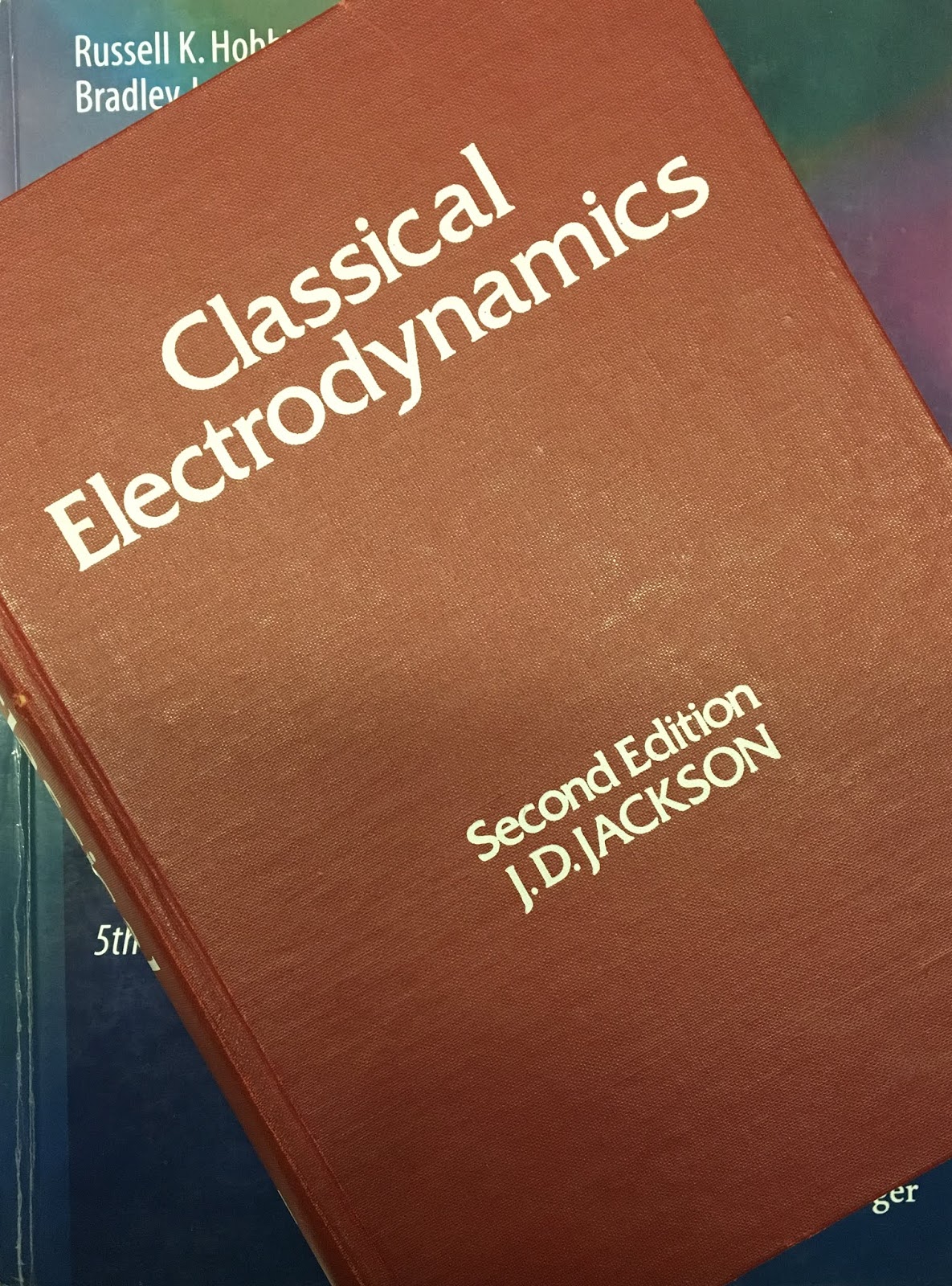
Their Chapter 1 begins by distinguishing between systematic and random errors. Bevington and Robinson illustrate the difference between accuracy and precision using a figure like this one:
 |
a) Precise but inaccurate data. b) Accurate but imprecise data.
|
In Chapter 2 of Data Reduction and Error Analysis, Bevington and Robinson introduce probability distributions.
Of the many probability distributions that are involved in the analysis of experimental data, three play a fundamental role: the binomial distribution [Appendix H in IPMB], the Poisson distribution [Appendix J], and the Gaussian distribution [Appendix I]. Of these, the Gaussian or normal error distribution is undoubtedly the most important in statistical analysis of data. Practically, it is useful because it seems to describe the distribution of random observations for many experiments, as well as describing the distributions obtained when we try to estimate the parameters of most other probability distributions.Here is something I didn’t realize about the Poisson distribution:
The Poisson distribution, like the bidomial distribution, is a discrete distribution. That is, it is defined only at integral values of the variable x, although the parameter μ [the mean] is a positive, real number.Figure J.1 of IPMB plots the Poisson distribution P(x) as a continuous function. I guess the plot should have been a histogram.
Chapter 3 addresses error analysis and propagation of error. Suppose you measure two quantities, x and y, each with an associated standard deviation σx and σy. Then you calculate a third quantity z(x,y). If x and y are uncorrelated, then the error propagation equation is
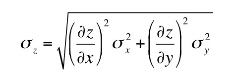

Bevington and Robinson derive the method of least squares in Chapter 4, covering much of the same ground as in Chapter 11 of IPMB. I particularly like the section titled A Warning About Statistics.
Equation (4.12) [relating the standard deviation of the mean to the standard deviation and the number of trails] might suggest that the error in the mean of a set of measurements xi can be reduced indefinitely by repeated measurements of xi. We should be aware of the limitations of this equation before assuming that an experimental result can be improved to any desired degree of accuracy if we are willing to do enough work. There are three main limitations to consider, those of available time and resources, those imposed by systematic errors, and those imposed by nonstatistical fluctuations.Russ and I mention Monte Carlo techniques—the topic of Chapter 5 in Data Reduction and Error Analysis—a couple times in IPMB. Then Bevington and Robinson show how to use least squares to fit to various functions: a line (Chapter 6), a polynomial (Chapter 7), and an arbitrary function (Chapter 8). In Chapter 8 the Marquardt method is introduced. Deriving this algorithm is too involved for this blog post, but Bevington and Robinson explain all the gory details. They also provide much insight about the method, such as in the section Comments on the Fits:
Although the Marquardt method is the most complex of the four fitting routines, it is also the clear winner for finding fits most directly and efficiently. It has the strong advantage of being reasonably insensitive of the starting values of the parameters, although in the peak-over-background example in Chapter 9, it does have difficulty when the starting parameters of the function for the peak are outside reasonable ranges. The Marquardt method also has the advantage over the grid- and gradient-search methods of providing an estimate of the full error matrix and better calculation of the diagonal errors.The rest of the book covers more technical issues that are not particularly relevant to IPMB. The appendix contains several computer programs written in Pascal. The OU library copy also contains a 5 1/2 inch floppy disk, which would have been useful 25 years ago but now is quaint.
Philip Bevington wrote the first edition of Data Reduction and Error Analysis in 1969, and it has become a classic. For many years he was a professor of physics at Case Western University, and died in 1980 at the young age of 47. A third edition was published in 2002. Download it here.
Friday, September 30, 2016
Rall's Equivalent Cylinder
Chapter 6 of Intermediate Physics for Medicine and Biology discusses nerve electrophysiology. In particular, Russ Hobbie and I derive the cable equation. This equation works great for a peripheral nerve with its single long cylindrical axon. In the brain, however, nerves end in branching networks of dendrites (see one of the famous drawings by Ramón y Cajal below). What equation describes the dendrites?
Wilfrid Rall answered this question by representing the dendrites as a branching network of fibers: the Rall model (Annals of the New York Academy of Sciences, Volume 96, Pages 1071–1092, 1962). Below I’
--> -->ll rederive the Rall model using the notation of IPMB. But—as I know some of you do not enjoy mathematics as much as I do—let me first describe his result qualitatively. Rall found that as you move along the dendritic tree, the fiber radius a gets smaller and smaller, but the number of fibers n gets larger and larger. Under one special condition, when na3/2 is constant, the voltage along the dendrites obeys THE SAME cable equation that governs a single axon. This only works if distance is measured in length constants instead of millimeters, and time in time constants instead of milliseconds. Dendritic networks don't always have na3/2 constant, but it is not a bad approximation, and provides valuable insight into how dendrites behave.
But instead of me explaining Rall’s goals, why not let Rall do so himself.
Now the math. First, let me review the cable model for a single axon, and then we will generalize the result to a network. The current ii along an axon is related to the potential v and the resistance per unit length ri by a form of Ohm's law
 (Eq. 6.48 in IPMB). If the current changes along the axon, it must enter or leave through the membrane, resulting in an equation of continuity
 (Eq. 6.49), where gm is the membrane conductance per unit area and cm is the membrane capacitance per unit area. Putting these two equations together and rearranging gives the cable equation
 The axon length constant is defined as
 and the time constant as
 so the cable equation becomes
 If we measure distance and time using the dimensionless variables X = x/λ and T = t/τ, the cable equation simplifies further to
 Now, let’s see how Rall generalized this to a branching network. Instead of having one fiber, assume you have a variable number that depends on position along the network, n(x). Furthermore, assume the radius of each individual fiber varies, a(x). The cable equation can be derived as before, but because ri now varies with position (ri = 1/nπa2σ, where σ is the intracellular conductivity), we pick up an extra term
 When I first looked at this equation, I thought “Aha! If ri is independent of x, the new term disappears and you get the plain old cable equation.”
It’s not quite that simple; λ also depends on position, so even without the extra term this is not the cable equation. Remember, we want to measure distance in the dimensionless variable X = x/λ, but λ depends on position, so the relationship between derivatives of x and derivatives of X is complicated
When I first looked at this equation, I thought “Aha! If ri is independent of x, the new term disappears and you get the plain old cable equation.”
It’s not quite that simple; λ also depends on position, so even without the extra term this is not the cable equation. Remember, we want to measure distance in the dimensionless variable X = x/λ, but λ depends on position, so the relationship between derivatives of x and derivatives of X is complicated

 In terms of the dimensionless variables X and T, the cable equation becomes
 If λri is constant along the axon, the ugly new term vanishes and you have the traditional cable equation. If you go back to the definition of ri and λ in terms of a and n, you find that this condition is equivalent to saying that na3/2 is constant along the network. If one fiber branches into two, the daughter fibers must each have a radius of 0.63 times the parent fiber radius. Dendritic trees that branch in this way act like a single fiber. This is Rall’s result: the Rall equivalent cylinder.
If you want to learn more about Rall’s work, read the book The Theoretical Foundation of Dendritic Function: Selected Papers of Wilfrid Rall with Commentaries, edited by Idan Segev, John Rinzel, and Gordon M. Shepherd. The foreword, by Terrence J. Sejnowski, says
 |
| A drawing of a dendritic tree, by Ramón y Cajal. |
--> -->ll rederive the Rall model using the notation of IPMB. But—as I know some of you do not enjoy mathematics as much as I do—let me first describe his result qualitatively. Rall found that as you move along the dendritic tree, the fiber radius a gets smaller and smaller, but the number of fibers n gets larger and larger. Under one special condition, when na3/2 is constant, the voltage along the dendrites obeys THE SAME cable equation that governs a single axon. This only works if distance is measured in length constants instead of millimeters, and time in time constants instead of milliseconds. Dendritic networks don't always have na3/2 constant, but it is not a bad approximation, and provides valuable insight into how dendrites behave.
But instead of me explaining Rall’s goals, why not let Rall do so himself.
In this paper, I propose to focus attention upon the branching dendritic trees that are characteristic of many neurons, and to consider the contribution such dendritic trees can be expected to make to the physiological properties of a whole neuron. More specifically, I shall present a mathematical theory relevant to the question: How does a neuron integrate various distributions of synaptic excitation and inhibition delivered to its soma-dendritic surface. A mathematical theory of such integration is needed to help fill a gap that exists between the mathematical theory of nerve membrane properties, on the one hand, and the mathematical theory of nerve nets and of populations of interacting neurons, on the other hand.I had the pleasure of knowing Rall when we both worked at the National Institutes of Health in the 1990s. He was trained as a physicist, and obtained his PhD from Yale. During World War II he worked on the Manhattan Project. He spent most of his career at NIH, and was a leader among scientists studying the theoretical electrophysiology of dendrites.
Rall receiving the Swartz Prize.


If you want to learn more about Rall’s work, read the book The Theoretical Foundation of Dendritic Function: Selected Papers of Wilfrid Rall with Commentaries, edited by Idan Segev, John Rinzel, and Gordon M. Shepherd. The foreword, by Terrence J. Sejnowski, says
The exploration of the electrical properties of dendrites by Wilfrid Rall provided many key insights into the computational resources of the neurons. Many of the papers in this collection are classics: dendrodendritic interactions in the olfactory bulb; nonlinear synaptic integration in motoneuron dendrites; active currents in pyramidal neuron apical dendrites. In each of these studies, insights arose from a conceptual leap, astute simplifying assumptions, and rigorous analysis. Looking back, one is impressed with the foresight shown by Rall in his choice of problems, with the elegance of his methods in attacking them, and with the impact that his conclusions have had for our current thinking. These papers deserve careful reading and rereading, for there are additional lessons in each of them that will reward the careful reader....It would be difficult to imagine the field of computational neuroscience today without the conceptual framework established over the last thirty years by Wil Rall, and for this we all owe him a great debt of gratitude.
Friday, September 23, 2016
Magneto-Aerotactic Bacteria Deliver Drug-Containing Nanoliposomes to Tumour Hypoxic Regions
In Chapter 8 of Intermediate Physics for Medicine and Biology, Russ Hobbie and I describe magnetotactic bacteria.
Several species of bacteria contain linear strings of up to 20 particles of magnetite, each about 50 nm on a side encased in a membrane (Frankelet al. 1979; Moskowitz 1995). Over a dozen different bacteria have been identified that synthesize these intracellular, membrane-bound particles or magnetosomes (Fig. 8.25). In the laboratory the bacteria align themselves with the local magnetic field. In the problems you will learn that there is sufficient magnetic material in each bacterium to align it with the earth’s field just like a compass needle. Because of the tilt of the earth’s field, bacteria in the wild can thereby distinguish up from down.I enjoy learning about the biology and physics of magnetotactic bacteria, but I never expected that they had anything to do with medicine. Then last month a paper published in Nature Nanotechnology discussed using these bacteria to treat cancer!
Other bacteria that live in oxygen-poor, sulfide-rich environments contain magnetosomes composed of greigite (Fe3S4), rather than magnetite (Fe3O4). In aquatic habitats, high concentrations of both kinds of magnetotactic bacteria are usually found near the oxic–anoxic transition zone (OATZ). In freshwater environments the OATZ is usually at the sediment–water interface. In marine environments it is displaced up into the water column. Since some bacteria prefer more oxygen and others prefer less, and they both have the same kind of propulsion and orientation mechanism, one wonders why one kind of bacterium is not swimming out of the environment favorable to it. Frankel and Bazylinski(1994) proposed that the magnetic field and the magnetosomes keep the organism aligned with the field, and that they change the direction in which their flagellum rotates to move in the direction that leads them to a more favorable concentration of some desired chemical.
Oxygen-depleted hypoxic regions in the tumour are generally resistant to therapies. Although nanocarriers have been used to deliver drugs, the targeting ratios have been very low. Here, we show that the magneto-aerotactic migration behaviour of magnetotactic bacteria, Magnetococcus marinus strain MC-1 (ref. 4), can be used to transport drug-loaded nanoliposomes into hypoxic regions of the tumour. In their natural environment, MC-1 cells, each containing a chain of magnetic iron-oxide nanocrystals, tend to swim along local magnetic field lines and towards low oxygen concentrations based on a two-state aerotactic sensing system. We show that when MC-1 cells bearing covalently bound drug-containing nanoliposomes were injected near the tumour in severe combined immunodeficient beige mice and magnetically guided, up to 55% of MC-1 cells penetrated into hypoxic regions of HCT116 colorectal xenografts. Approximately 70 drug-loaded nanoliposomes were attached to each MC-1 cell. Our results suggest that harnessing swarms of microorganisms exhibiting magneto-aerotactic behaviour can significantly improve the therapeutic index of various nanocarriers in tumour hypoxic regions.The IOP website physicsworld.com published an article by Belle Dumé describing this study. It begins
Bacteria that respond to magnetic fields and low oxygen levels may soon join the fight against cancer. Researchers in Canada have done experiments that show how magneto-aerotactic bacteria can be used to deliver drugs to hard-to-reach parts of tumours. With further development, the method could be used to treat a variety of solid tumours, which account for roughly 85% of all cancers.A similar article, also by Dumé, can be found on medicalphysicsweb.com
As cancer cells proliferate, they consume large amounts of oxygen. This results in oxygen-poor regions in a tumour. It is notoriously difficult to treat these hypoxic regions using conventional pharmaceutical nanocarriers, such as liposomes, micelles and polymeric nanoparticles.Pretty cool stuff.
Now, a team led by Sylvain Martel of the NanoRobotics Laboratory at the Polytechnique Montréal has developed a method that exploits the magnetotactic bacteria Magnetoccus marinus (MC-1) to overcome this problem.
Subscribe to:
Posts (Atom)

