Friday, July 3, 2009

Sync

Sync, By Steven Strogatz, superimposed on Intermediate Physics for Medicine and Biology.
Sync, By Steven Strogatz.
In the October 17, 2008 entry to this blog, I discussed Steven Strogatz’s textbook Nonlinear Dynamics and Chaos, which Russ Hobbie and I cite in Intermediate Physics for Medicine and Biology. Toward the end of that entry, I mentioned that reading Strogatz’s other book,  Sync, was “on my list of things to do.” Well, jobs often sit on my to-do list for a long time, but they eventually get done. This week I finished Sync, a fascinating book about “how order emerges from chaos in the universe, nature, and daily life.” It is an unusual mathematics book, because I don’t recall seeing a single equation. Nevertheless, Strogatz tells a charming tale of his contributions, and that of many others, to nonlinear dynamics. Russ added a citation to Sync to our chapter on Feedback and Control when we were preparing the 4th edition of Intermediate Physics for Medicine and Biology:
Strogatz (2003) discusses phase-resetting and other nonlinear phenomena in an engaging and nonmathematical manner.
The Geometry of Biological Time, by Art Winfree, superimposed on Intermediate Physics for Medicine and Biology.
The Geometry of Biological Time,
by Art Winfree.
Chapter Eight of Strogatz’s book, “Sync in Three Dimensions,” is my favorite. Here he describes how he first discovered the work of Art Winfree, his “mentor, inspiration, friend.”
I walked across the street to Heffer’s Bookstore to browse the books on biomathematics… As I scanned the shelves, with my head tilting sideways, one title popped out at me:  The Geometry of Biological Time. Now that was a weird coincidence. My senior thesis on DNA had been subtitled An Essay on Geometric Biology. I thought I had invented that odd juxtaposition, geometry next to biology. But the book’s author, someone named Arthur T. Winfree, from the biology department at Purdue University, had obviously connected them first.
Strogatz then relates how he corresponded with Winfree, and ended up working with him at Purdue in the summer of 1982. He quotes Winfree’s letters, often written in what Strogatz calls “idiosyncratic code.” This characteristic style brought back memories of my own correspondence with Winfree. Although we only met in person once, I recall us exchanging many emails about cardiac dynamics, with his emails all in that same idiosyncratic code. As I read Winfree’s letters to Strogatz, I found myself thinking “yes, that is exactly the way Winfree would have said it.”

When Time Breaks Down: The Three Dimensional Dynamics of Electrochemical Waves and Cardiac Arrhythmias, by Arthur Winfee, superimposed on Intermediate Physics for Medicine and Biology.
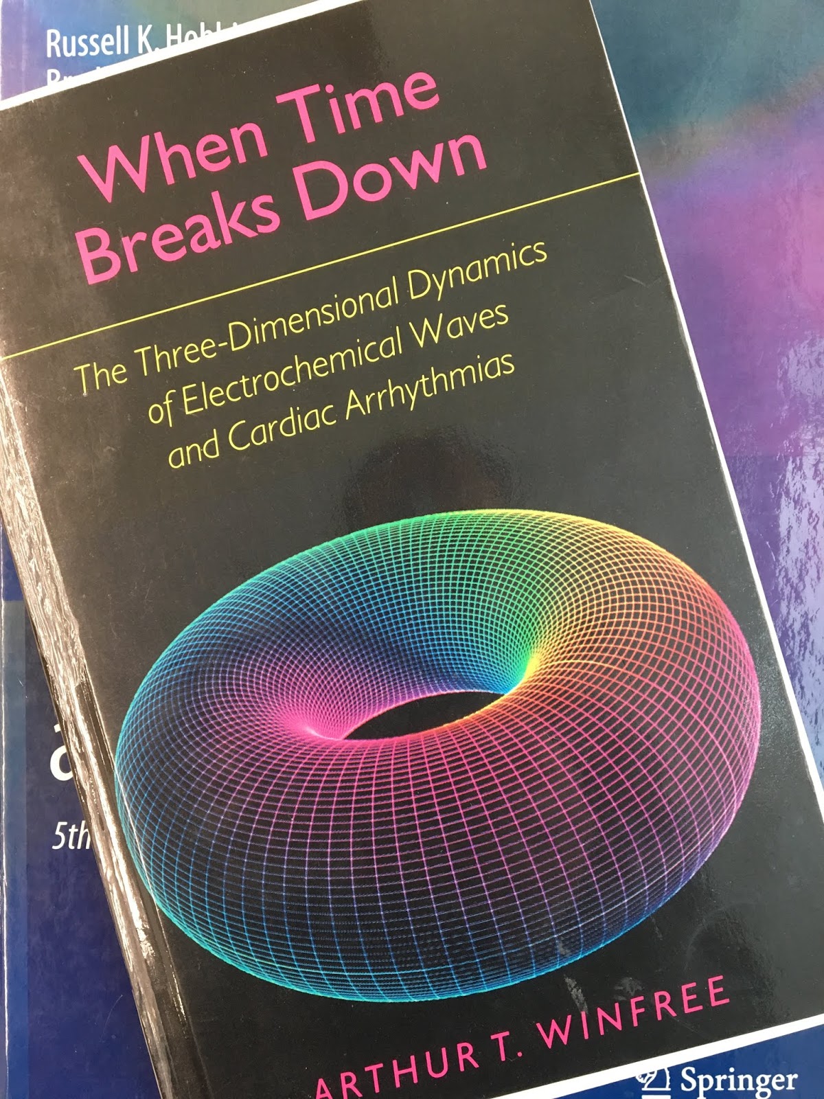
When Time Breaks Down,
by Art Winfree.
I had my own encounter with a Winfree book that influenced my early career. For me, it was not The Geometry of Biological Time, but Winfree’s other influential text, When Time Breaks Down: The Three Dimensional Dynamics of Electrochemical Waves and Cardiac Arrhythmias. I read the book in the spring of 1991. (I remember the time precisely, because I recall turning the pages of the book with one hand, while holding my newborn daughter Kathy with the other.) I was soon performing calculations of reentrant wave propagation in cardiac tissue, similar to the dynamics described in When Time Breaks Down. I worked at the National Institutes of Health at the time, and a summer student, Josh Saypol, and I performed a calculation of reentry induction using the bidomain model to test a prediction that Winfree had made in a chapter of the book Cardiac Electrophysiology: From Cell to Bedside (1990). His help was invaluable in interpreting our results, and for getting a preliminary note (The Formation of a Re-entrant Action Potential Wave Front in Tissue with Unequal Anisotropy Ratios) published in the just-started International Journal of Bifurcation and Chaos (Volume 1, Pages 927–928, 1991).

Strogatz describes Winfree’s untimely death in the epilog of Sync.

Tragically, Art Winfree died on November 5, 2002, at age 60, seven months after being diagnosed with brain cancer. He helped me with this book at every stage, even when he was conscious only for a few hours a day. Though he did not live to see it published, he knew that it would be dedicated to him.
For more about Winfree’s career, see his website (still available through the University of Arizona), the obituary Strogatz wrote for the Society for Industrial and Applied Mathematics, another by Leon Glass in Nature, and also one in the New York Times.

I described my own interactions with Winfree, and some of his contributions to cardiac electrophysiology, in my paper
Art Winfree and the Bidomain Model of Cardiac Tissue, published in a special issue of the Journal of Theoretical Biology dedicated to his memory (Volume 230, Pages 445449, 2004). Other particularly interesting contributions to that issue, full of delightful Winfree anecdotes, were the article by his daughter Rachael, and the article by George Oster.

I thoroughly enjoyed Sync. It is a fine introduction to the mathematics of synchronization and nonlinear dynamics. (Don’t, however, consult the book to learn how lasers work!) Sync ends with a lovely paragraph that explains what motivates scientists:

For reasons I wish I understood, the spectacle of sync strikes a chord in us, somewhere deep in our souls. It’s a wonderful and terrifying thing. Unlike many other phenomena, the witnessing of it touches people at a primal level. Maybe we instinctively realize that if we ever find the source of spontaneous order, we will have discovered the secret of the universe.
Alas, my to-do list never gets any shorter. Strogatz has a new book coming out next month, The Calculus of Friendship: What a Teacher and a Student Learned about Life while Corresponding about Math, and I plan to read it as soon as I get a bit of spare time.

Friday, June 26, 2009

Physics Meets Biology

Readers of the 4th edition of Intermediate Physics for Medicine and Biology may find a news feature by Jonathan Knight published in the September 19, 2002 issue of Nature interesting. The article “Physics Meets Biology: Bridging the Culture Gap” (Volume 419, Page 244–246) begins
“In late July, several dozen physicists with an interest in biology gathered at the Colorado mountain resort of Snowmass for a birthday celebration. Hans Frauenfelder, a physicist who began studying proteins decades ago, turned 80 this year. But unofficially, the physicists were celebrating something else—a growing feeling that their discipline’s mindset will be crucial to reaping the harvest of biologys postgenomic era.
It continues:
“Biology today is where physics was at the beginning of the twentieth century,” observes José Onuchic, who is the co-director of the new Center for Theoretical Biological Physics (CTBP) at the University of California, San Diego. It is faced with a lot of facts that need an explanation.

Physicists believe that they can help, bringing a strong background in theory and the modeling of complexity to nudge the study of molecules and cells in a fresh direction. What has been all too rare in biology is the symbiosis between theory and experiment that is routine in physics, says Laura Garwin, director of research affairs at Harvard Universitys Bauer Center for Genomics Research, who has made her own transition to biology—she was once Natures physical-sciences editor.
The article concludes
“Onuchic believes that immersing young physicists in the culture of biology is the key. At the CTBP, postdocs train in both disciplines simultaneously, developing projects that involve two labs, one in biology and one in physics. They attend two sets of group meetings, and so learn the language and mentality of both disciplines at the same time. They get inside the culture of the two fields, Onuchic says. They get comfortable with the vocabulary and the journals. Life in both labs is more important than any classes you can take.

Time will tell whether the new generation of biological physicists avoid becoming the lonely children of biology. But for now, the prospects look bright. We have always been the odd kids in the playground, says Onuchic. But we never gave up, and now we are becoming very popular.”

Friday, June 19, 2009

Resource Letter PFBi-1: Physical Frontiers in Biology

Eugenie Mielczarek of George Mason University published “Resource Letter PFBi-1: Physical Frontiers in Biology” in the American Journal of Physics (Volume 74, Pages 375–381, 2006). The fourth edition of Intermediate Physics for Medicine and Biology was one of 39 books listed in the letter.

What are Resource Letters? They are collections of references that are published periodically by the American Journal of Physics.
Resource Letters are guides for college and university physicists, astronomers, and other scientists to literature, websites, and other teaching aids. Each Resource Letter focuses on a particular topic and is intended to help teachers improve course content in a specific field of physics or to introduce nonspecialists to this field.
Mielczarek’s Resource Letter discusses topics that will be of interest to readers of Intermediate Physics for Medicine and Biology.
This Resource Letter provides a guide to the literature on physical frontiers in biology. Books and review articles are cited as well as journal articles for the following topics: cells and cellular mats; conformational dynamics/folding; electrostatics; enzymes, proteins, and molecular machines; material-biomineralization; miscellaneous topics; nanoparticles and nanobiotechnology; neuroscience; photosynthesis; quantum mechanics theory; scale and energy; spectroscopy and microscopy: experiments and instrumentation; single-molecule dynamics; and water and hydrogen-bonded solvents. A list of web resources and videotapes is also given.
The letter begins with a fascinating 3-page overview of the role of physics in biology. For instance, Mielczarek asks the question

Which principles govern life? Dutifully the physicist might answer—the organizing of electrons into their lowest energy states, forcing molecules and groups of molecules into specific configurations. But be cautious: this simplistic answer implies an isolated system in equilibrium. It conceals the dynamics of life, which require a continuous input of matter and energy. Cells, tissues and organisms are dependent upon energy refreshment.
Iron, Nature's Universal Element:  Why People Need Iron and Animals Make Magnets,  by Eugenie Mielczarek, superimposed on Intermediate Physics for Medicine and Biology.
Iron, Nature's Universal Element:
Why People Need Iron and Animals Make Magnets
,
by Eugenie Mielczarek.
Readers who enjoy Intermediate Physics for Medicine and Biology will probably find Mielczarek's Resource Letter to be a valuable... well, resource. They may also enjoy her book Iron, Nature's Universal Element: Why People Need Iron and Animals Make Magnets.

Friday, June 12, 2009

The Magnetic Field of a Single Axon

When I was in graduate school, working in John Wikswo’s lab at Vanderbilt University, I calculated and measured the magnetic field of a single nerve axon. The calculation makes a nice, although slightly advanced, homework problem for Chapter 8 of the 4th edition of Intermediate Physics for Medicine and Biology.
Section 8.2

Problem 14.5 Use Ampere’s law to calculate the magnetic field produced by a nerve axon.

(a) First, solve Problem 30 of Chapter 7 to obtain the electrical potential inside (Vi) and outside (Vo) an axon. The solution will be in terms of the modified Bessel functions I0(kr) and K0(kr), where k is a spatial frequency and r is the radial distance from the center of the axon. Assume the axon has a radius a.

(b) Find the axial component of the current density, J, both inside and outside the axon using Jiz = − σi dVi/dz and Joz = σo dVo/dz, where σi and σo are the intracellular and extracellular conductivities (Eqs. 6.16b and 6.26).

(c) Integrate Jiz over the axon cross-section to get the total intracellular current. Then integrate Joz over an annulus from a to the radius r, to get the “return current.”

(d) Use Ampere’s law (Eq. 8.9) to calculate the magnetic field. Take the line integral of Ampere's law as a closed loop of radius r concentric with the axon (r greater than a). The current enclosed by this loop is simply the sum of the intracellular and return currents calculated in (c).

In part (c), you will need the Bessel function integrals
∫ I0(x) x dx = x I1(x)
∫ K0(x) x dx = - x K1(x) .
To check your solution, see Eq. A13 of “The Magnetic Field of a Single Axon” (Roth and Wikswo, Biophysical Journal, Volume 48, Pages 93–109, 1985). However, that paper uses complex exponentials whereas Problem 30 of Chapter 7 uses sines and cosines, introducing a slight difference between your expression and that in Eq. A13 of the Roth and Wikswo paper.

Classical Electrodynamics, by John David Jackson, superimposed on Intermediate Physics for Medicine and Biology.
Classical Electrodynamics,
by John David Jackson.
I recall the day I derived this expression for the magnetic field. I was puzzled because another graduate student in Wikswo's lab, James Woosley, had derived a different expression for the magnetic field of an axon using the Biot-Savart law (Sec. 8.2.3). How could there be two seemingly different expressions for the magnetic field? Previous discussions with Prof. John Barach had given me a hint. He had derived two expressions for the magnetic field produced by a battery in a bucket of saline, using either Ampere’s law or the Biot-Savart law, and showed that they were the same (he eventually published this in The Effect of Ohmic Return Current on Biomagnetic Fields, Journal of Theoretical Biology, Volume 125, Pages 187191, 1987). I worried about this problem for some time, until one evening (September 22, 1983; Wikswo insisted that I keep careful records in my lab notebook) I was working on my electricity and magnetism homework and found the solution staring at me: Eq. 3.147 in Jacksons famous textbook Classical Electrodynamics (here I quote the current 3rd Edition, but at the time I was using my now tattered 2nd Edition with the red cover). This equation defines the Wronskian condition for Bessel functions

I0(x) K1(x) + K0(x) I1(x) = 1/x .

I didn't have all my work at home, so I remember riding my bike (I didn
t yet own a car) back to the lab in the rain so I could check if the Wronskian would resolve the difference between my expression and Woosleys. It did; the two expressions were equivalent (in my usually dry notebook, I wrote HA! It works). You can calculate the magnetic field using either Amperes law or the Biot-Savart law, and you get the same result. To see how these two equations predict the same magnetic field in a slightly easier case (like that considered by Barach), solve Problem 13 of Chapter 8 in the 4th edition of Intermediate Physics for Medicine and Biology.

For those of you interested in Woosley
s expression, you can find its derivation in The Magnetic Field of a Single Axon: A Volume Conductor Model (Woosley, Roth, and Wikswo, Mathematical Biosciences, Volume 76, Pages 136, 1985). In particular, they state on page 13
If we... rearrange terms, and use a relation which can be derived from the Wronskian... we can show that... Equation (45), derived from Amperes law, is identical to... Equation (36), derived from the law of Biot and Savart.
Vanderbilt Research Notebook 4, Page 21, September 22, 1983.

Friday, June 5, 2009

Ichiji Tasaki (1910-2009)

Ichiji Tasaki (1910–2009) died January 4 in Bethesda, Maryland. Tasaki was known for his discovery in 1939 of saltatory conduction of action potentials in a myelinated nerve axon. You can learn more about myelinated fibers and saltatory conduction in the 4th edition of Intermediate Physics for Medicine and Biology.

Tasaki had a long and fascinating career in science. His life is described in an obituary published in the May 2009 issue of Neuroscience Research. He is also featured in an article of the NIH Record, the weekly newsletter for employees of the National Institutes of Health.

I knew Tasaki when I was working at NIH in the 1990s. Late in his career he worked with my friend Peter Basser in the National Institute of Child Health and Human Development. I recall him working every day in his laboratory, despite being in his 80s, with his wife as his assistant. He led a fascinating life. His best known research on saltatory conduction was performed in Japan just before and during World War II. After the war, he spent over 50 years at NIH.

Basser describes Tasaki as “a scientist’s scientist, never afraid to question current dogma, always digging deeper to discover the truth.” Congressman Chris van Hollen of Maryland paid tribute to Tasaki a few months before he died, beginning
Madam Speaker, I rise today to recognize the outstanding achievements of my constituent Dr. Ichiji Tasaki. Dr. Tasaki has worked at the National Institutes of Health for 54 years, since November 1953, and has made invaluable contributions to the scientific community.

Friday, May 29, 2009

Deep Brain Stimulation

In Chapter 7 of the 4th edition of Intermediate Physics for Medicine and Biology, Russ Hobbie and I describe electrical stimulation (Section 7.10, pages 192–196), including excitation of peripheral nerves (Problems 7.38–7.41) and cardiac pacemakers. Another increasingly important procedure is deep brain stimulation. On May 21, Medtronic announced Food and Drug Administration approval of two new models of the Activa stimulator for use in the United States to treat Parkinson’s disease and essential tremor. This device is similar to a pacemaker, but electrodes are implanted in the brain instead of the heart. The detailed electrophysiological mechanism is still unknown, but repetitive stimulation of certain structures deep in the brain provides dramatic relief to some patients with movement disorders. The new Activa RC and PC stimulators have features not available in older models, such as the RC’s rechargeable battery.
 
A friend of mine, Frans Gielen, has worked on deep brain stimulation at the Medtronic Bakken Research Centre in Maastricht, the Netherlands. Frans was a post doc when I was a graduate student at Vanderbilt University, working in the laboratory of John Wikswo; we both worked on measuring the magnetic field of nerves and muscle fibers (for instance, see Gielen, Roth and Wikswo, “Capabilities of a Toroid-Amplifier System for Magnetic Measurement of Current in Biological Tissue,” IEEE Transactions on Biomedical Engineering, Volume 33, Pages 910
–921, 1986). Frans is considered at Medtronic as the architect of the Medtronic Activa Tremor Control Therapy. Known fondly while in Wikswo’s lab as that crazy Dutchman, when he left Vanderbilt we were not surprised that Frans would make important contributions to Medtronic.

For more about deep brain stimulation, two review articles are
Deep Brain Stimulation for Parkinson's Disease(Benabid AL, Current Opinion in Neurobiology, Volume 13, Pages 696–706 2003) and Uncovering the Mechanism(s) of Action of Deep Brain Stimulation: Activation, Inhibition, or Both(McIntyre CC, Savasta M, Kerkerian-Le Goff L, Vitek JL, Clinical Neurophysiology, Volume 115, Pages 1239–1248, 2004).

Deep Brain Stimlation,
by Jamie Talan.
For those wanting to read about deep brain stimulation from the patient's perspective, see Deep Brain Stimulation: A New Treatment Shows Promise in the Most Difficult Cases, by Jamie Talan. In the Prologue, Talan writes
On March 14, 1997, the U.S. Food and Drug Administration held a hearing on the use of deep brain stimulation (DBS) as a treatment for essential tremor and Parkinson’s disease. By that time, excitement about this technology, which could restore a body to its rightful state of controlled movement, had spread through brain research laboratories and neurology clinics around the world. Desperate patients with all kinds of movement disorders had heard about deep brain stimulation, too, and they were clamoring for access to the treatment.

On this day in March, two American patients, Maurice Long and George Shafer, were standing before an advisory panel commissioned by the FDA to study the benefits and risks of deep brain stimulation. Long and Shafer were among the 83 people with essential tremor and 113 people with Parkinson's tremor who had undergone deep brain stimulation in a large clinical trial. The FDA-approved study was sponsored by Medtronic, the Minneapolis-based company that supplied the simulating electrodes for the trial. Founded in 1949 to usher in a new technology called cardiac pacing, Medtronic had made the first implantable heart pacemaker. Now the company was in the middle of an international push on another frontier: the brain seemed to be as receptive to electrical stimulation as the heart.

Friday, May 22, 2009

Using Logarithmic Transformations When Fitting Allometric Data

In the 4th edition of Intermediate Physics for Medicine and Biology, Russ Hobbie and I discuss least squares fitting. A homework problem at the end of Chapter 11 (see page 321) asks the student to fit some data to a power law.
Problem 11 Consider the data given in Problem 2.36 relating molecular weight M and molecular radius R. Assume the radius is determined from the molecular weight by a power law: R = B Mn. Fit the data to this expression to determine B and n. Hint: Take logarithms of both sides of the equation.
The solution manual (available at the book’s website, contact one of the authors for the password) outlines how taking logarithms makes the problem linear, so a simple linear least squares fit gives the solution R = 0.0534 M0.371.

However, inquisitive students may ask “what if I don’t follow the hint, and do a least squares fit to the original power law without taking logarithms. Do I get the same result?” This becomes a more difficult problem, since you must now make a nonlinear least squares fit. Nevertheless, I solved the problem this way (using a terribly inefficient iterative guess-and-check method) and found R = 0.0619 M0.358.

Which solution is correct? Gary Packard and Thomas Boardman, both from Colorado State University, address this question in their paper “A Comparison of Methods for Fitting Allometric Equations to Field Metabolic Rates of Animals” (Journal of Comparative Physiology, B, Volume 179, Pages 175–182, 2009), and find that

the discrepancies could be caused by four sources of bias acting singly or in combination to cause exponents (and coefficients) estimated by back-transformation from logarithms to be inaccurate and misleading. First, influential outliers may go undetected in some analyses ... owing to the altered relationship between X and Y variables that accompanies logarithmic transformation ... Second, the use of logarithmic transformations may result in the fitting of mathematical functions (i.e., two-parameter power functions) that are poor descriptors of data in the original scale ... Third, a two-parameter power function ... fitted to the original data by least squares invokes a statistical model with additive error Y = aXb + e and predicts arithmetic means for Y whereas a straight line fitted to logarithmic transformations of the data by least squares invokes an underlying model with multiplicative error Y = aXb 10e and predicts geometric means for the response variable ... And fourth, linear regression on nonlinear transformations like logarithms may introduce further bias into analyses by the unequal weighting of large and small values for both X and Y...

Conversion to logs results in an overall compression of the distributions for both the Y- and X-variables, but the compression is greater at the high ends of the scales than at the low ends... Consequently, linear regression on transformations gives unduly large influence to small values for Y and X and unduly small influence to large ones... This disparate influence is apparent in plots of back-transformations against the backdrop of data in their original scales, where the location of data for the largest animals had little apparent influence on fits of the lines.
Their paper concludes
Why transform? Log transformations have a long history of use in allometric research... and have been justified on grounds ranging from linearizing data to achieving better distributions for purposes of graphical display... However, most of the reasons for making such transformations disappeared with the advent of powerful PCs and sophisticated software for graphics and statistics. Indeed, the only ongoing application for log transformations in allometric research is in adjusting (‘‘stabilizing’’) distributions when residuals from analyses performed in the original scale are not distributed normally and/or when variances are not constant at all values for X. Assuming that log transformations actually linearize the data and produce the desired distributions, the regression of log Y on log X will yield evidence for a dependency between Y and X values in their original state, and statistical comparisons can be made with other samples that also are expressed in logarithmic form. However, interpretations about patterns of variation of the variables in the arithmetic domain seldom are warranted... because transformation fundamentally alters the relationship between the predictor and response variables. Interest typically is in patterns of variation of data expressed in an arithmetic scale, so this is the scale in which allometric analyses need to be performed if it is at all possible to do so.

Implications for allometric research. Accumulating evidence from the field of biology... and beyond... gives cause for concern about the accuracy and reliability of allometric equations that have been estimated in the traditional way... This concern has special bearing on the current debate about the true’’ exponent for scaling of metabolism to body mass because exponents of 2/3 and 3/4 need both to be viewed with some skepticism. The aforementioned evidence also indicates that the traditional approach to allometric analysis may need to be abandoned in favor of a new research paradigm that will prevent future studies from being compromised by the insidious effects of logarithmic transformations.
In the above quote, many of the ...s indicate important references that I skipped to save space.

Packard and Boardman make a persuasive case that you might want to ignore our hint at the end of Problem 11. However, if you do ignore it, you had better be prepared to do nonlinear least squares fitting. See Sec. 11.2, Nonlinear Least Squares, in our book to get started.

For more about this subject, see Packard
s letter to the editor in the Journal of Theoretical Biology (Volume 257, Pages 515–518, 2009). Also, Russ Hobbie has a paper submitted to the journal Ecology that discusses a similar issue with exponential, rather than power law, least squares fits (Single pool exponential decomposition models: Potential pitfalls in their use in ecological studies). Russs coatuhors are E. Carol Adair and Sarah E. Hobbie (Russs daughter), both of the University of Minnesota in Saint Paul.

Friday, May 15, 2009

Current Injection into a Two-Dimensional Anisotropic Bidomain

Twenty years ago this month, Nestor Sepulveda, John Wikswo, and I published a calculation of the transmembrane potential induced when a point electrode passes current into cardiac tissue, as might happen when pacing the heart (“Current Injection into a Two-Dimensional Anisotropic Bidomain,” Biophysical Journal, Volume 55, Pages 987–999, 1989). When we wrote the paper, Sepulveda was a Research Assistant Professor and I had just gotten my PhD and was starting a one-year post doc in Wikswo’s laboratory at Vanderbilt University. We used a mathematical model of the electrical properties of cardiac tissue called the bidomain model, which was relatively new at that time. In Chapter 7 of the 4th edition of Intermediate Physics for Medicine and Biology, Russ Hobbie and I describe this result.
The bidomain has been used to understand the response of cardiac tissue to stimulation... [Sepulveda et al.’s] simulation explains a remarkable experimental observation. Although the speed of the wave front is greater along the fibers than perpendicular to them, if the stimulation is well above threshold, the wave front originates farther from the cathode in the direction perpendicular to the fibers—the direction in which the speed of propagation is slower. The simulations show that this is due to the anisotropy in conductivity. This is called the “dog-bone” shape of the virtual cathode. It can rotate with depth in the myocardium because the myocardial fibers change orientation. The difference in anisotropy accentuates the effect of a region of hyperpolarization surrounding the depolarization region produced by a cathode electrode. Strong point stimulation can also produce reentry waves that can interfere with the desired pacing effect.
The calculation was possible because Sepulveda had developed a finite element computer program that could solve the bidomain equations: a system of two coupled partial differential equations. Meanwhile, Wikswo was performing experiments on dog hearts with collaborators at the Vanderbilt Hospital, and had observed that the wave fronts originate from a spot farther from the electrode in the direction perpendicular to the fibers than in the direction parallel to them (Virtual Cathode Effects during Stimulation of Cardiac-Muscle 2-Dimensional In Vivo Experiments,Circulation Research, Volume 68, Pages 513–530, 1991). As soon as Sepulveda performed the calculation, they realized that it would explain Wikswos data.

I remember being so surprised hyperpolarization would be produced just a millimeter or two away from a cathode that I quietly slipped into my office and developed a Fourier method to check Sepulveda
s finite element calculation. I got the same result: regions of hyperpolarization adjacent to the cathode. After our publication, six years passed before the prediction of hyperpolarized regions was verified experimentally, by three groups simultaneously including researchers in Wikswos lab (Virtual Electrodes in Cardiac Tissue: A Common Mechanism for Anodal and Cathodal Stimulation, Biophysical Journal, Volume 69, Pages 21952210, 1995). During these years—when I was working at the National Institutes of HealthJosh Saypol, an undergraduate summer student, and I showed that the hyperpolarization could have an important effect: it could lead to reentry, a type of cardiac arrhythmia (“A Mechanism for Anisotropic Reentry in Electrically Active Tissue, Journal of Cardiovascular Electrophysiology, Volume 3, Pages 558566, 1992). For a simple, visual, and non-mathematical introduction to these ideas, see my paper in the Online Journal of Cardiology.

Our original publication in 1989 has now been cited in the literature 200 times. It remains one of my most cited papers (although, to be honest, I had less to do with the research than Sepulveda and Wikswo did), and is one of my favorites.

Friday, May 8, 2009

Color Vision

Color vision is one topic from biological physics that Russ Hobbie and I do not discuss in the 4th edition of Intermediate Physics for Medicine and Biology. Why? Well, the book is already rather long, and it is printed in black and white. To do justice to this topic, one really needs color pictures.

The Last Man Who  Knew Everything,  by Andrew Robinson, superimposed on Intermediate Physics for Medicine and Biology.
The Last Man Who
Knew Everything,
by Andrew Robinson.
The history of color vision is fascinating, in part because it illustrates the role that physics and physicists can play in the life sciences. The fundamental idea of trichromatic color vision was developed by two giants of 19th century physics, Thomas Young and Hermann von Helmholtz. Young was a fascinating intellectual, who Andrew Robinson describes in his book The Last Man Who Knew Everything: Thomas Young, the Anonymous Genius Who Proved Newton Wrong and Deciphered the Rosetta Stone, Among Other Surprising Feats. Helmholtz was a leading figure in early German physics (see: Hermann von Helmholtz and the Foundations of Nineteenth-Century Science).

The Young-Helmholtz theory postulates three types of photoreceptors in the eye, corresponding to three different colors of light: red (long wavelength), green (intermediate wavelength), and blue (short wavelength). Other colors can be formed by a mixture of these three. For instance, yellow is a combination of red and green (which amazes me, because yellow does not look anything like what you might expect from a red-green mixture). You can make yellow light two ways: a single wavelength of light intermediate between red and green so it excites both the red and green receptors (their response curves overlap), or by two wavelengths—one pure red and one pure green
mixed together. Your eye can’t tell the difference: in each case the red and green receptors are both excited. However, you could easily tell which is which using a prism or diffraction grating. Cyan is a mixture of green and blue (and cyan does indeed look like what you might call blue-green). Magenta is a mixture of blue and red, and is a particularly interesting case because it is not one of the colors of the rainbow: you could not, for instance, have a magenta laser, because a laser outputs a single wavelength of light—one color—but in order to produce magenta you need to excite both the red and blue receptors without exciting the green receptor. There is no way to do this without using at least two wavelengths. Of course, if you mix all three colors (that is, excite all three receptors simultaneously) you get white light.

Color mixing is much easier to understand if you can visualize it. I suggest going to one of the excellent color mixing applets on the internet, such as this one, or this one. If none of this sounds much like what you learned when mixing paint in kindergarten, it’s because there you were really doing color subtraction, rather than color addition.

Once you understand color mixing, you can understand color blindness. The most common type is red-green color blindness, where either the red or green receptor is absent. If the green receptor is not present, you cannot distinguish red from green or yellow (both excite only the red receptor), although you can still distinguish red from blue or magenta. Not sure if you are colorblind? There are many websites available that offer tests, including this one and this one. Not all animals have trichomatic vision. Your dog has only two receptors, making her a dichromat.

Another physicist that worked on color vision was James Clerk Maxwell, who is best remembered for his monumental work on electromagnetic theory (“Maxwell’s Equations”), as well as his work on the kinetic theory of gasses. But he also studied color vision by using wheels painted with more than one color, which when spun would produce a color mixture. Maxwell also produced the first color photograph.
The Feynman Lectures on Physics, by Richard Feynman, superimposed on Intermediate Physics for Medicine and Biology.
The Feynman Lectures on Physics,
by Richard Feynman.

We should keep in mind this admonition from Richard Feynman in Volume 1 of his famous  The Feynman Lectures on Physics: “Color is not a question of the physics of light itself. Color is a sensation, and the sensation for different colors is different in different circumstances.” If you dont believe this, see this optical illusion. You can even play tricks on your eye by creating afterimages like this one. Color vision is a fascinating subject, and a great example of the interaction between physics and physiology.

Friday, May 1, 2009

Paul Lauterbur

This week we celebrate the 80th anniversary of the birth of Paul Lauterbur (May 6, 1929–March 27, 2007), co-winner with Peter Mansfield of the 2003 Nobel Prize in Physiology or Medicine “for their discoveries concerning magnetic resonance imaging. Lauterbur’s contribution was the introduction of magnetic field gradients, so that differences in frequency could be used to localize the spins. In Sec. 18.9 of the 4th edition of Intermediate Physics for Medicine and Biology, Russ Hobbie and I describe this technique.
Creation of the [magnetic resonance] images requires the application of gradients in the static magnetic field Bz which cause the Larmor frequency to vary with position. The first gradient is applied in the z direction [the same direction as the static magnetic field] during the pi/2 pulse so that only the spins in a slice in the patient are selected (nutated into the xy plane). Slice selection is followed by gradients of Bz in the x and y directions. These also change the Larmor frequency. If the gradient is applied during the readout, the Larmor frequency of the signal varies as Bz varies with position. If the gradient is applied before the readout, it causes a position-dependent phase shift in the signal which can be detected.
Lauterbur grew up in Sidney, Ohio. He attended college at Case Institute of Technology, now part of Case Western Reserve University in Cleveland, where he majored in chemistry. He obtained his PhD in Chemistry in 1962 from the University of Pittsburgh. He was a Professor at the State University of New York at Stony Brook from 1969-1985, during which time he published his landmark paper Image Formation by Induced Local Interactions: Examples Employing Nuclear Magnetic Resonance, (Nature, Volume 242, Pages 190–191, 1973). In an interesting story, Lauterbur came up with the idea of using gradients to do magnetic resonance imaging while eating a hamburger in a Big Boy restaurant.
Principles of Magnetic Resonance Imaging: A Signal Processing Perspective, by Liang and Lauterbur, superimposed on Intermeidate Physics for Medicine and Biology.
Principles of Magnetic Resonance Imaging:
A Signal Processing Perspective,
by Liang and Lauterbur.

You can learn more about magnetic resonance imaging by reading Lauterbur’s book (with Zhi-Pei Liang) Principles of Magnetic Resonance Imaging: A Signal Processing Perspective. If looking for a briefer introduction, consult Chapter 18 of Intermediate Physics for Medicine and Biology. Be sure to use the 4th edition if you want to learn about recent developments, such as functional MRI and diffusion tensor imaging.